Lecture
We have had many cases to see how important the basic numerical characteristics of random variables are in probability theory: mathematical expectation and variance for one random variable, mathematical expectation and the correlation matrix for a system of random variables. The art of using numerical characteristics, leaving as far as possible the laws of distribution, is the basis of applied probability theory. The apparatus of numerical characteristics is a very flexible and powerful apparatus, which makes it relatively easy to solve many practical problems.
A completely similar apparatus is used in the theory of random functions. For random functions, the simplest basic characteristics similar to the numerical characteristics of random variables are also introduced, and the rules of actions with these characteristics are established. Such a device is sufficient to solve many practical problems.
In contrast to the numerical characteristics of random variables that provide certain numbers, the characteristics of random functions are, in general, not numbers, but functions.
Expectation of random function  is defined as follows. Consider the cross section of a random function
  with fixed
  . In this section we have the usual random variable; we define its expectation. Obviously, in the general case it depends on
  i.e. it represents some function
  :
:
 . (15.3.1)
Thus, the mathematical expectation of a random function  called non-random function
  which for every argument value
  equal to the mathematical expectation of the corresponding cross section of a random function.
In terms of meaning, the expectation of a random function is some average function, around which the concrete implementations of the random function vary in various ways.
In fig. 15.3.1 thin lines show the implementation of a random function, a bold line is its expectation.
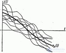
Fig. 15.3.1.
Similarly, the variance of a random function is determined.
Variance random function  called non-random function
  whose value for each
  equal to the variance of the corresponding cross section of the random function:
 . (15.3.2)
Variance of a random function at each  characterizes the scatter of possible implementations of a random function relative to the mean, in other words, the “degree of randomness” of a random function.
Obviously  there is a non-negative function. Taking from it the square root, we obtain the function
  - standard deviation of the random function:
 . (15.3.3)
Expectation and variance are very important characteristics of a random function; however, these characteristics are not enough to describe the main features of the random function. To see this, consider two random functions.  and
and  , visually depicted by the family of realizations in fig. 15.3.2 and 15.3.3.
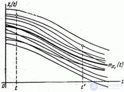
Fig. 15.3.2.
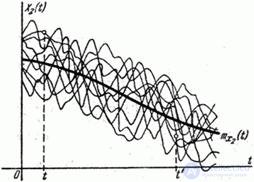
Fig. 15.3.3.
Do random functions  and
and  approximately the same expectation and variance; however, the nature of these random functions is dramatically different. For random function
  (fig. 15.3.2) is characterized by a smooth, gradual change. If, for example, at the point
  random function
  took a value significantly higher than the average, it is very likely that at the point
  it will also take a value greater than average. For random function
  characterized by a pronounced dependence between its values at different
  . In contrast, a random function
  (fig. 15.3.3) has a sharply oscillating character with irregular, erratic fluctuations. Such a random function is characterized by a rapid decay of the dependence between its values with increasing distance along
  between them.
Obviously, the internal structure of both random processes is completely different, but this difference is not captured by either expectation or dispersion; for its description it is necessary to maintain a special characteristic. This characteristic is called the correlation function (otherwise, the autocorrelation function). The correlation function characterizes the degree of dependence between the cross sections of a random function relating to different  .
.
Let there be a random function  (fig. 15.3.4); Consider two of its sections relating to different points:
  and
and  i.e. two random variables
  and
and  . Obviously, with close values
  and
and  magnitudes
  and
and  are closely related: if the value
  took some value, then the value
  is likely to take a value close to it. It is also obvious that with an increase in the interval between sections
  ,
,  magnitude dependence
  and
and  should generally decrease.
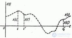
Fig. 15.3.4.
Degree of dependence  and
and  can be largely characterized by their correlation point; obviously, it is a function of two arguments
  and
and  . This function is called the correlation function.
Thus, the correlation function of the random function  called the non-random function of two arguments
  which with every pair of values
  ,
,  equal to the correlation moment of the corresponding sections of the random function:
 , (15.3.4)
Where
 ,
,  .
.
Let's return to examples of random functions.  and
and  (fig. 15.3.2 and 15.3.3). We see now that with the same expectation and variance, random functions
  and
and  have completely different correlation functions. Correlation function of a random function
  decreases slowly as the gap increases
  ; on the contrary, the correlation function of a random function
  decreases rapidly with increasing this gap.
Find out what the correlation function turns to.  when her arguments match. Putting
  , we have:
 , (15.3.5)
i.e.  the correlation function is drawn to the variance of the random function.
Thus, the need for dispersion as a separate characteristic of a random function disappears: as the main characteristics of a random function, it suffices to consider its expectation and correlation function.
Since the correlation moment of two random variables  and
and  does not depend on the sequence in which these quantities are considered, the correlation function is symmetric with respect to its arguments, i.e. it does not change when the arguments change places:
 . (15.3.6)
If to draw the correlation function  in the form of a surface, then this surface will be symmetric about the vertical plane
  passing through the bisector of the angle
  (fig. 15.3.5).
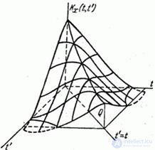
Fig. 15.3.5.
We note that the properties of the correlation function naturally follow from the properties of the correlation matrix of a system of random variables. Indeed, we replace the approximately random function.  system
  random variables
  . By increasing
  and, accordingly, the reduction of the intervals between the arguments of the correlation matrix of the system, which is a table of two inputs, in the limit goes into the function of two continuously changing arguments, which has similar properties. The symmetry property of the correlation matrix with respect to the main diagonal is transferred to the symmetry property of the correlation function (15.3.6). On the main diagonal of the correlation matrix are the variances of random variables; similarly with
  correlation function
  turns into a dispersion
  .
.
In practice, if you want to build a correlation function of a random function  , usually come in the following way: set by a number of equally spaced argument values and build the correlation matrix of the resulting system of random variables. This matrix is nothing but a table of values of the correlation function for a rectangular grid of argument values on the plane.
  . Further, by interpolating or approximating, we can construct a function of two arguments
  .
.
Instead of the correlation function  You can use the normalized correlation function:
 , (15.3.7)
which is the correlation coefficient of the quantities  ,
,  . The normalized correlation function is similar to the normalized correlation matrix of a system of random variables. With
  normalized correlation function is equal to one:
 . (15.3.8)
Let us find out how the basic characteristics of a random function change during elementary operations on it: when adding a nonrandom term and when multiplying by a nonrandom factor. These non-random terms and factors can be both constant values and, in general, functions.  .
.
Let's add to the random function  nonrandom term
  . Get a new random function:
 . (15.3.9)
By the theorem of addition of mathematical expectations:
 , (15.3.10)
that is, when a nonrandom term is added to a random function, the same nonrandom term is added to its expectation.
Define the correlation function of a random function  :
:


 , (15.3.11)
that is, by adding a nonrandom term, the correlation function of a random function does not change.
Multiply random function  to a non-random factor
  :
:
 . (15.3.12)
Carrying a non-random value  as a sign of mathematical expectation, we have:
 , (15.3.13)
that is, when a random function is multiplied by a nonrandom factor, its expectation is multiplied by the same factor.
Determine the correlation function:

 , (15.3.14)
that is, when multiplying a random function by a nonrandom function  its correlation function is multiplied by
  .
.
In particular, when  (not dependent on
  ), the correlation function is multiplied by
  .
.
Using the derived properties of the characteristics of random functions, in some cases it is possible to significantly simplify operations with them. In particular, when it is necessary to investigate the correlation function or the variance of a random function, you can advance from it to the so-called centered function:
 . (3/15/15)
The expectation of a centered function is identically zero, and its correlation function coincides with the correlation function of a random function  :
:
 . (3/15/16)
In the study of issues related to the correlation properties of random functions, in the future we will always move from random functions to the corresponding centered functions, marking this with  at the top of the function sign.
Sometimes, besides centering, rationing of random functions is also applied. Normalized is called a random function of the form:
 . (15.3.17)
Correlation function of the normalized random function  equals
 , (15.3.18)
and its variance is one.
Comments
To leave a comment
Probability theory. Mathematical Statistics and Stochastic Analysis
Terms: Probability theory. Mathematical Statistics and Stochastic Analysis