Correlation and regression analysis. Linear correlation

Content

1. Methods for studying the relationship of socio-economic phenomena using correlation-regressive analysis
2. Linear correlation

General idea of ​​the correlation analysis

The forms and types of relations existing between phenomena are very diverse in their classification. The subject of statistics are only those of them that are quantitative in nature and are studied using quantitative methods. Consider the method of correlation and regression analysis, which is fundamental in the study of the relationship of phenomena.

This method contains two of its constituent parts - correlation analysis and regression analysis. Correlation analysis is a quantitative method for determining the closeness and direction of the relationship between sampling variables. Regression analysis is a quantitative method for determining the type of mathematical function in a causal relationship between variables.

To assess the strength of the connection in the theory of correlation, the Cheddock scale of English statistics is used: weak - from 0.1 to 0.3; moderate - from 0.3 to 0.5; noticeable - from 0.5 to 0.7; high - from 0.7 to 0.9; very high (strong) - from 0.9 to 1.0. It is used further in the examples on the topic.

Linear correlation

This correlation characterizes the linear relationship in the variations of variables. It can be paired (two correlating variables) or multiple (more than two variables), direct or inverse - positive or negative, when the variables vary, respectively, in the same or different directions.

If the variables are quantitative and equivalent in their independent observations with their total then the most important empirical measures of the closeness of their linear interrelationship are the direct correlation coefficient of Austrian psychologist G.T. 1936).

The pairwise correlation coefficient of Fechner signs determines the consistency of directions in the individual deviations of variables and from their medium and . It is equal to the ratio of the difference of the sums of coinciding ( ) and mismatched ( ) pairs of characters in deviations and to the sum of these amounts:

The value of Kf varies from -1 to +1. Summation in (1) is made according to the observations which are not listed in amounts for the sake of simplification. If any one deviation or then it is not included in the calculation. If both deviations are zero at once: , then such a case is considered to be coincident in signs and is part of . In table 12.1. shows the preparation of data for the calculation (1).

Table 12.1 Data for the calculation of the Fechner coefficient.

By (1) we have Kf = (3 - 2) / (3 + 2) = 0.20 . The direction of interconnection in variations !! The average number of employees | number of employees]] and the volume of turnover - positive (straight): signs in deviations and and in the majority (in 3 cases out of 5) coincide with each other. The tightness of the relationship of variables on the Cheddock scale is weak.

The coefficients of the paired, pure (private) and multiple (total) linear Pearson correlations, in contrast to the Fechner coefficient, take into account not only the signs, but also the magnitudes of the deviations of the variables. For their calculation using different methods. So, according to the direct counting method based on ungrouped data, the Pearson pair correlation coefficient is:

This coefficient also varies from -1 to +1. In the presence of several variables, the Pearson multiple (cumulative) linear correlation coefficient is calculated. For three variables x, y, z, it has the form

This coefficient varies from 0 to 1. If to eliminate (completely eliminate or fix at a constant level) the effect on and then their “general” connection will turn into “pure”, forming a pure (private) Pearson linear correlation coefficient:

This ratio varies from -1 to +1. The squares of the correlation coefficients (2) - (4) are called coefficients (indices) of determination - respectively paired, clean (private), multiple (total):

Each of the coefficients of determination varies from 0 to 1 and estimates the degree of variational certainty in the linear relationship of variables, showing the fraction of variation of one variable (y) due to the variation of the other (s) - x and y. The multidimensional case of the presence of more than three variables is not considered here.

According to the development of English statistics R.E. Fisher (1890-1962), the statistical significance of the pairwise and pure (particular) Pearson correlation coefficients is checked in the case of their normal distribution, based on -the distribution of English statistics vs Gosset (pseudonym "Student"; 1876-1937) with a given level of probabilistic significance and the degree of freedom where - number of links (factor variables). 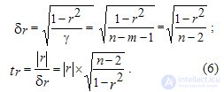For the pair coefficient we have its rms error and the actual value Student Criteria:

For net correlation coefficient when calculating it instead of (n-2) must be taken because in this case there is m = 2 (two factor variables x and z). For a large number n> 100, instead of (n-2) or (n-3) in (6), we can take n, neglecting the accuracy of the calculation.

If tr> ttabl. , then the pair correlation coefficient - total or pure is statistically significant, and for tr ≤ ttable. - insignificant.

The significance of the multiple correlation coefficient R is checked by F - Fisher criterion by calculating its actual value

When FR> Ftabl. the coefficient R is considered significant with a given level of significance a and the available degrees of freedom and , and at Fr≤ Ftabl - insignificant.

In the aggregates of a large volume n> 100, the normal distribution law is applied directly (tabulated Laplace-Sheppard function) to assess the significance of all Pearson coefficients instead of the criteria t and F.

Finally, if the Pearson coefficients do not obey the normal law, then Z - Fisher criterion is used as a criterion of their significance, which is not considered here.

Conditional calculation example (2) - (7) given in table. 12.2, where the initial data of Table 12.1 are taken with the addition of the third variable z - the size of the total area of ​​the store (in 100 sq. M).

Table 12.2. Data preparation for calculating Pearson correlation coefficients

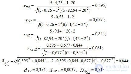
According to (2) - (5), the Pearson linear correlation coefficients are:

The relationship of the variables x and y is positive, but not close, making up the value of their pair correlation coefficient and on pure - size and was rated on the Cheddok scale, respectively, as "noticeable" and "weak."

The coefficients of determination dxy = 0.354 and dxy.z = 0.0037 indicate that the variation of y (turnover) is due to a linear variation of x (the number of employees) by 35.4% in their total interrelation and in the net interrelation - only by 0.37% . This situation is due to the significant effect on x and y of the third variable z - the total area occupied by stores. The tightness of its relationship with them is respectively rxz = 0.677 and ryz = 0.844 .

The coefficient of multiple (cumulative) correlations of the three variables shows that the tightness of the linear relationship x and z c y is R = 0.844 , estimated by the Cheddock scale as “high”, and the coefficient of multiple determination is D = 0.713 , indicating that 71.3 % of all variations of y (commodity turnover) are due to the cumulative effect of variables x and z on it. The remaining 28.7% are due to the impact on y of other factors or the curvilinear connection of the variables y, x, z .

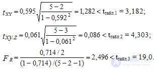
To assess the significance of correlation coefficients, take the significance level . According to the initial data, we have degrees of freedom for and for . According to the theoretical table we find, respectively, ttabl.1. = 3.182 and table.2. = 4.303. For the F-criterion we have and and on the table we find Ftabl. = 19.0. The actual values ​​of each criterion for (6) and (7) are equal to:

All calculated criteria are less than their tabular values: all Pearson correlation coefficients are statistically insignificant.

See also

• Correlation and regression analysis. Linear correlation
• Tables The value of the Laplace function f (x), tγ, q Critical points of the distribution of χ2 and Student