Lecture
The task of determining the distribution law of a function of several random arguments is much more complicated than a similar problem for a function of one argument. Here we present a general method for solving this problem for the simplest case of a function of two arguments.
There is a system of two continuous random variables.  with distribution density
  . Random value
  associated with
  and
and  functional dependence:
 .
.
It is required to find the distribution law  .
.
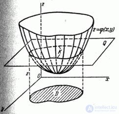
To solve the problem, we use a geometrical interpretation similar to the one we used in the case of a single argument. Function  it’s no longer a curve, but a surface (fig. 12.4.1).

Fig. 12.4.1.
Find the distribution function of  :
:
 . (12.4.1)
Draw a plane  parallel to the plane
  , on distance
  from her. This plane will cross the surface.
  on some curve
  . Design the curve
  on the plane
  . This projection, whose equation
  will divide the plane
  into two areas; for one of them is the height of the surface above the plane
  will be less, and for another - more
  . Denote
  the area for which this height is less
  . To satisfy inequality (12.4.1), a random point
  obviously should get into the area
  ; Consequently,
 . (12.4.2)
In the expression (12.4.2) value  enters implicitly through the limits of integration.
Differentiating  by
by  , we obtain the distribution density
  :
:
 .
.
Knowing the specific type of function  , you can express the limits of integration through
  and write the expression
  explicitly.
In order to find the distribution law of the function of two arguments, there is no need to construct a surface each time.  , just as it is done in fig. 12.4.1, and cross it by a plane parallel to
  . In practice, it is enough to build on the plane
  curve whose equation
  , be aware of which side of this curve
  and for what
  and integrate by region
  , for which
  .
.
Example. System of quantities  subject to the distribution law with density
  . Magnitude
  there is a product of quantities
  :
:
 .
.
Find the density distribution  .
.
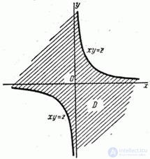
Decision. Let's set some value  and build on the plane
  curve whose equation
  (fig. 12.4.2). This is a hyperbole whose asymptotes coincide with the axes of coordinates. Region
  in fig. 12.4.2 shaded.

Fig. 12.4.2.
Distribution function of magnitude  has the form:
 .
.
Differentiating this expression by  , we have:
 . (12.4.3)
Comments
To leave a comment
Probability theory. Mathematical Statistics and Stochastic Analysis
Terms: Probability theory. Mathematical Statistics and Stochastic Analysis