15.1. Theory of random functions. Concept of random function

So far, in our course on probability theory, the main subject of research has been random variables. The random variable is characterized by the fact that as a result of the experiment it takes some one, previously unknown, but the only value. Examples of such random variables are: the abscissa of the point of impact when fired; radio range error at one, single measurement range; horizontal error at one shot, etc.

Limiting ourselves to the consideration of such individual random variables, we studied random phenomena as if “in statics”, in some fixed constant conditions of a separate experience.

However, such an elementary approach to the study of random phenomena in a number of practical problems is clearly insufficient. In practice, one often has to deal with random variables that continuously change in the process of experience. Examples of such random variables are: the error of the radio range finder during continuous measurement of the changing range; lead angle with continuous aiming at a moving target; the deviation of the trajectory of the controlled projectile from the theoretical in the process of control or homing.

Such random variables, which change in the course of experience, we will, unlike ordinary random variables, call random functions.

The study of such random phenomena, in which randomness manifests itself in the form of a process, is dealt with by a special branch of the theory of probability — the theory of random functions (otherwise, the theory of random or stochastic processes). This science can be figuratively called "the dynamics of random phenomena."

The theory of random functions is the newest section of probability theory, which has developed mainly in the last two or three decades. At present, this theory continues to evolve and improve at a very fast pace. This is due to the immediate requirements of practice, in particular the need to solve a number of technical problems. It is known that in recent times systems with automated control have become more and more common. Accordingly, all the great demands are made on the theoretical basis of this type of technology - the theory of automatic control. The development of this theory is impossible without the analysis of errors that inevitably accompany control processes, which always occur under conditions of continuously acting random disturbances (the so-called “interferences”). These disturbances are, by their nature, random functions. In order to rationally select the design parameters of the control system, it is necessary to study its response to continuously acting random perturbations, and the only apparatus suitable for such a study is the apparatus of the theory of random functions.

In this chapter, we will introduce the basic concepts of this theory and the general formulation of a number of practical problems requiring the application of the theory of random functions. In addition, here will be outlined the general rules of operating with characteristics of random functions, similar to the rules of operating with the numerical characteristics of ordinary random variables.

The first of the basic concepts with which we have to deal is the very concept of a random function. This concept is as wide and rich as the concept of a random variable, as far as the mathematical concepts of a variable quantity and a function are wider and richer than the concept of a constant quantity.

Recall the definition of a random variable. A random variable is a quantity that, as a result of experience, may take one or another value, it is not known in advance what exactly. We give a similar definition of a random function.

A random function is a function that, as a result of experience, can take one or another specific form, it is not known in advance what exactly.

The specific form taken by a random function as a result of experience is called the realization of a random function. If we make a group of experiments on a random function, then we will get a group or a “family” of implementations of this function.

We give some examples of random functions.

Example 1. A bomber on a combat course has theoretically constant airspeed . In fact, its speed fluctuates around this average nominal value and is a random function of time. Flying on a combat course can be viewed as an experience in which the random function accepts a specific implementation (Fig. 15.1.1).

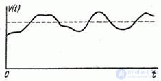
Fig. 15.1.1.

From experience to experience, the view of implementation changes. If a self-recording device is installed on the plane, then in each flight it will record a new, different from the others, implementation of the random function. As a result of several flights, you can get a family of realizations of a random function. (fig. 15.1.2).

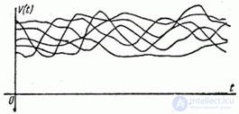
Fig. 15.1.2.

Example 2 is the deviation of the center of mass of the projectile from the theoretical trajectory, that is, a random function of time (Fig. 15.1.3).

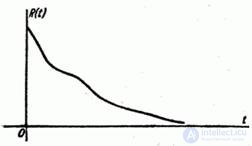
Fig. 15.1.3.

In the same experience, random functions of time are, for example, projectile overload , attack angle etc.

Example 3. When shooting from an airplane at an airplane, the crosshair for a certain period of time must be continuously combined with the goal of following it. The target tracking operation is accompanied by errors - the so-called aiming errors (Fig. 15.1.4).

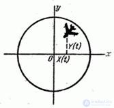
Fig. 15.1.4.

Horizontal and vertical aiming errors in the process of aiming are constantly changing and are two random functions. and . The implementation of these random functions can be obtained as a result of the decryption of the photos of the photo-gun, which photographs the target during the entire tracking process.

The number of examples of random functions found in the technique could be increased without limit. Indeed, in any case, when we are dealing with a continuously operating system (measurement, control, guidance, regulation), when analyzing the accuracy of this system, we have to take into account the presence of random influences (interference). Both the interferences themselves and the system response caused by them are random functions of time.

So far, we have been talking only about random functions whose argument is time . In a number of practical tasks, there are random functions that depend not on time, but on other arguments. For example, the strength characteristics of a non-uniform rod can be considered as random functions of the abscissa of the cross section . Air temperature in various layers of the atmosphere can be considered as a random function of altitude. .

In practice, there are also random functions that depend not on one argument, but on several. For example, aerological data characterizing the state of the atmosphere (temperature, pressure, wind) are, in general, random functions of four arguments: three coordinates and time .

In this course, we will consider only random functions of one argument. Since this argument is most often time, we will denote it by the letter . In addition, we agree, as a rule, to denote random functions in capital letters unlike non-random functions .

Consider some random function. . Suppose that it is produced independent experiments, which resulted in implementations (Fig. 15.1.5).

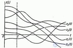
Fig. 15.1.5.

Denote them according to the experience number. .

Each implementation, obviously, is an ordinary (non-random) function. Thus, as a result of each experience, the random function turns into a normal, non-random function.

Now let's fix some value of the argument. and see what happens to a random function. . Obviously, it will turn into a random variable in the usual sense of the word. We agree to call this random variable the cross section of a random function corresponding to . If you hold a "cross section" of the family of implementations for a given (fig. 15.1.5) we will get random values at experiences.

We see that a random function combines the features of a random variable and a function. If we fix the value of the argument, it becomes a normal random variable; as a result of each experience, it turns into a normal (non-random) function.

In the course of the further presentation, we will often alternately consider the same function. then as a random function, then as a random variable, depending on whether it is considered on the entire range of change or at its fixed value.