Lecture
Previous  we addressed the issue of estimating an unknown parameter
  one number. Such an assessment is called "point". In a number of tasks it is required not only to find for the parameter suitable numerical value, but also to assess its accuracy and reliability. It is required to know - to what errors the replacement of the parameter can lead its point estimate
  and with what degree of confidence can we expect that these errors will not go beyond certain limits?
Such tasks are especially relevant with a small number of observations, when the point estimate largely random and approximate replacement on can lead to serious errors.
To give an idea of the accuracy and reliability of the assessment , in mathematical statistics use the so-called confidence intervals and confidence probabilities.
Let for parameter unbiased estimate obtained from experience . We want to evaluate the possible error. Assign some fairly large probability  (eg,
(eg, 
 or
or  ) such that an event with probability can be considered almost reliable, and find such a value
  , for which
 . (14.3.1)
Then the range of practically possible values of the error that occurs when replacing on , will be  ; large errors in absolute magnitude will appear only with a small probability
  .
.
Rewrite (14.3.1) in the form:
 . (14.3.2)
Equality (14.3.2) means that with probability unknown parameter value falls into the interval
 . (14.3.3)
It should be noted one thing. Previously, we have repeatedly considered the probability of a random variable falling into a given non-random interval. Here it is different: the value not random, but random  . Randomly its position on the x-axis, determined by its center ; the length of the interval is also random
  because the magnitude It is calculated, as a rule, by experimental data. Therefore, in this case it is better to interpret the value not like the probability of "hitting" the point in the interval , but as the probability that a random interval will cover the point (fig. 14.3.1).
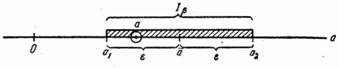
Fig. 14.3.1.
Probability it is accepted to call confidence probability, and the interval - confidence interval. Interval boundaries :  and
and  are called confidential boundaries.
We give another interpretation of the concept of a confidence interval: it can be considered as an interval of parameter values compatible with the experimental data and do not contradict them. Indeed, if we agree to consider an event with probability almost impossible then those parameter values for which  , it is necessary to recognize contradicting experimental data, and those for which
  compatible with them.
Let us turn to the question of finding confidential boundaries.  and
and  .
.
Let for parameter there is an unbiased estimate . If we knew the distribution law , the task of finding a confidence interval would be quite simple: it would be enough to find such a value , for which
.
The difficulty is that the distribution law estimates depends on the law of distribution of magnitude  and, therefore, from its unknown parameters (in particular, from the parameter itself). ).
To circumvent this difficulty, you can apply the following roughly approximate method: replace in the expression for unknown parameters of their point estimates. With a relatively large number of experiments  (order
  a) this method usually gives results with satisfactory accuracy.
As an example, consider the confidence interval problem for the expectation.
Let produced independent experiments on a random variable whose characteristics are mathematical expectation  and variance
  - unknown. Estimates for these parameters are obtained:
 ;
;  . (14.3.4)
Required to build a confidence interval  corresponding to the confidence level for mathematical expectation magnitudes .
In solving this problem, we use the fact that  represents the sum independent identically distributed random variables
  and, according to the central limit theorem, with a sufficiently large its distribution law is close to normal. In practice, even with a relatively small number of terms (about
  a) the distribution law of the sum can be approximately considered normal. We will proceed from the fact that distributed according to normal law. The characteristics of this law — expectation and variance — are equal, respectively. and
  (see ch. 13
  13.3). Suppose the value we know and find the value
  for which
 . (14.3.5)
Applying the formula (6.3.5) of Chapter 6, we express the probability on the left side (14.3.5) through the normal distribution function
 . (14.3.6)
Where  - standard deviation of assessment .
From the equation

find the value :
 , (14.3.7)
Where  - inverse function
  , i.e., the value of the argument for which the normal distribution function is
  .
.
Dispersion through which the value is expressed  , we are not exactly known; as its approximate value, you can use the estimate (14.3.4) and put approximately:
 . (14.3.8)
Thus, the problem of constructing a confidence interval, which is equal to:
 , (14.3.9)
Where determined by the formula (14.3.7).
To avoid when calculating inverse interpolation in function tables , it is convenient to make a special table (see table. 14.3.1), where the values of

depending on the . Magnitude  determines for the normal law the number of standard quadratic deviations that need to be postponed to the right and left of the center of dispersion in order that the probability of getting into the resulting section is equal to .
Through value confidence interval is expressed as:
 .
.
Table 14.3.1
|
|
|
|
|
|
|
|
0.80 | 1.282 | 0.86 | 1,475 | 0.91 | 1.694 | 0.97 | 2,169 |
0.81 | 1,310 | 0.87 | 1.513 | 0.92 | 1,750 | 0.98 | 2,325 |
0.82 | 1,340 | 0.88 | 1.554 | 0.93 | 1.810 | 0.99 | 2.576 |
0.83 | 1,371 | 0.89 | 1,597 | 0.94 | 1,880 | 0.9973 | 3,000 |
0.84 | 1,404 | 0.90 | 1,643 | 0.95 | 1,960 | 0.999 | 3.290 |
0.85 | 1,439 | 0.96 | 2,053 |
Example 1. Produced 20 experiments on the value ; the results are shown in table 14.3.2.
Table 14.3.2
|
|
|
|
|
|
|
|
one | 10.5 | 6 | 10.6 | eleven | 10.6 | sixteen | 10.9 |
2 | 10.8 | 7 | 10.9 | 12 | 11.3 | 17 | 10.8 |
3 | 11.2 | eight | 11.0 | 13 | 10.5 | 18 | 10.7 |
four | 10.9 | 9 | 10.3 | 14 | 10.7 | nineteen | 10.9 |
five | 10.4 | ten | 10.8 | 15 | 10.8 | 20 | 11.0 |
Required to find a rating for mathematical expectation magnitudes and build a confidence interval corresponding to the confidence probability  .
.
Decision. We have:
 .
.
Choosing a starting point  , using the third formula (14.2.14) we find the unbiased estimate
  :
:
 ;
;
 .
.
According to table 14.3.1 we find  ;
;
 .
.
Confidence limits:
 ;
;
 .
.
Confidence interval:
 .
.
Parameter values lying in this interval are consistent with the experimental data given in table 14.3.2.
In a similar way, a confidence interval can also be constructed for dispersion.
Let produced independent experiments on a random variable with unknown parameters and and for dispersion unbiased estimate received:
, (14.3.11)
Where
.
It is required to approximately build a confidence interval for the variance.
From the formula (14.3.11) it can be seen that represents the sum random variables of the form  . These values are not independent, since any of them includes the value depending on everyone else. However, it can be shown that by increasing the distribution law of their sum also approaches normal. Practically at
  it can already be considered normal.
Suppose that this is so, and we find the characteristics of this law: expectation and variance. Since the evaluation - unbiased, then
 .
.
Variance calculation  associated with relatively complex calculations, so we give its expression without output:
 , (14.3.12)
Where  - the fourth central moment of magnitude .
To use this expression, you need to substitute the values in it and (at least approximate). Instead you can use his assessment . In principle, the fourth central point You can also replace it with an estimate, for example, a value of the form:
 (14.3.13)
but such a replacement will give extremely low accuracy, since in general, with a limited number of experiments, moments of high order will be determined with large errors. However, in practice it often happens that the type of distribution law known in advance: only its parameters are unknown. Then you can try to express through .
Take the most frequent case when distributed according to normal law. Then its fourth central moment is expressed in terms of variance (see Ch. 6 6.2):
 ,
,
and the formula (14.3.12) gives

or
 . (14.3.14)
Replacing in (14.3.14) the unknown his assessment , we get:
 (14.3.15)
from where
 . (14.3.16)
Moment can be expressed through also in some other cases where the distribution of the magnitude It is not normal, but its appearance is known. For example, for the law of uniform density (see Chapter 5) we have:
 ;
;  ,
,
Where  - the interval at which the law is given. Consequently,
 .
.
According to the formula (14.3.12) we get:
 ,
,
where we find approximately
 . (14.3.17)
In cases where the type of distribution law unknown, with estimated value  it is recommended to use the formula (14.3.16), if there are no special grounds for believing that this law is very different from normal (it has a noticeable positive or negative kurtosis).
If approximate value obtained in one way or another, it is possible to build a confidence interval for the variance, in the same way as we built it for the expectation:
 , (14.3.18)
where is the value depending on a given probability is in table 14.3.1.
Example 2. Find approximately 80% confidence interval for the variance of a random variable in the conditions of example 1, if it is known that distributed according to a law close to normal.
Decision. The value remains the same as in example 1:
.
According to the formula (14.3.16)
 .
.
According to the formula (14.3.18) we find the confidence interval:
 .
.
The corresponding interval of values of the standard deviation:  .
.


Comments
To leave a comment
Probability theory. Mathematical Statistics and Stochastic Analysis
Terms: Probability theory. Mathematical Statistics and Stochastic Analysis