Lecture
The distribution function of a system of two random variables  called the probability of joint fulfillment of two inequalities
  and
and  :
:
 . (8.2.1)
If we use for the geometric interpretation of the system the image of a random point, then the distribution function  there is nothing like the probability of hitting a random point
  in an infinite quadrant with a vertex at a point
  lying to the left and below it (Fig. 8.2.1). In a similar interpretation, the distribution function of one random variable
  - we denote it
  - represents the probability of hitting a random point in the half-plane, bounded to the right by the abscissa
  (Fig. 8.2.2); single value distribution function
  - probability of hitting the half-plane bounded by ordinate y (Fig. 8.2.3).
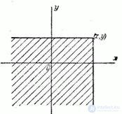
Fig. 8.2.1
AT  5.2 we gave the main properties of the distribution function
  for one random variable. We formulate similar properties for the distribution function of a system of random variables and again use the geometric interpretation to illustrate these properties.
1. Distribution function  there is a non-decreasing function of both its arguments, i.e.
at  ;
;
at  .
.
In this property of the function  can be clearly seen using the geometric interpretation of the distribution function as the probability of falling into a quadrant with vertex
  (Fig. 8.2.1). Indeed, increasing
  (by shifting the right edge of the quadrant to the right) or by increasing
  (by shifting the upper boundary upward), we obviously cannot reduce the probability of falling into this quadrant.
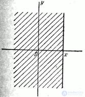
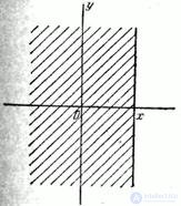
Fig. 8.2.2 Figure 8.2.3
2. Everywhere  the distribution function is zero:
 .
.
In this property we clearly see, unlimitedly pushing the right edge of the quadrant to the left  or down its upper limit
  or doing it simultaneously with both boundaries; while the probability of hitting the quadrant tends to zero.
3. With one of the arguments equal to  , the function of the distributed system becomes the distribution function of a random variable corresponding to another argument:
 ,
,
Where  - respectively, the distribution function of the random, the distribution function of values
  and
and  .
.
This property of the distribution function can be clearly seen by shifting one or another of the boundaries of the quadrant by  ; while in the limit the quadrant turns into a half-plane, the probability of falling into which is the distribution function of one of the quantities included in the system.
4. If both arguments are equal  , the distribution function of the system is equal to one:
 .
.
Indeed, with  ,
,  quadrant with vertex
  in the limit turns into the whole plane
  , hit in which there is a reliable event.
When considering the laws of distribution of individual random variables (Chapter 5), we derived an expression for the probability of a random variable falling within a given segment. We expressed this probability both through the distribution function and through the distribution density.
In a similar way for a system of two random variables is the question of the probability of hitting a random point  within the specified area
  on surface
  (Fig.8.2.4).
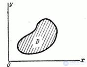
Fig. 8.2.4
Let's arrange an event consisting in hitting a random point  to the area
  denote by symbol
  .
.
The probability of hitting a random point in a given area is expressed most simply in the case when this area is a rectangle with sides parallel to the coordinate axes.
Express through the distribution function of the system the probability of hitting a random point  into a rectangle
  limited by abscissas
  and
and  and ordinates
  and
and  (Fig. 8.2.5).
In this case, it should be agreed where we will refer the borders of the rectangle. In the same way as we did for one random variable, we agree to include in the rectangle  its lower and left borders and not include the upper and right. Then event
  will be equivalent to the product of two events:
  and
and  . Express the probability of this event through the distribution function of the system. To do this, look at the plane
  four infinite quadrants with vertices at points
  ;
;  ;
;  and
and  (Fig. 8.2.6).
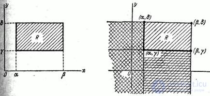
Fig. 8.2.5. Fig. 8.2.6
Obviously, the probability of hitting the rectangle  equal to the probability of falling into the quadrant
  minus the probability of hitting the quadrant
  minus the probability of hitting the quadrant
  plus probability of hitting the quadrant
  (since we twice deducted the probability of falling into this quadrant). From here we obtain a formula expressing the probability of hitting a rectangle through the distribution function of the system:
 . (8.2.2)
Later, when the notion of the distribution density of the system is introduced, we derive a formula for the probability that a random point will fall into a region of arbitrary shape.
Comments
To leave a comment
Probability theory. Mathematical Statistics and Stochastic Analysis
Terms: Probability theory. Mathematical Statistics and Stochastic Analysis