17.8. Characterization of an ergodic stationary random function in one implementation

Consider the stationary random function which has an ergodic property, and suppose that we have only one implementation of this random function, but on a sufficiently large time interval . For an ergodic stationary random function, one implementation of a sufficiently long duration is practically equivalent (in terms of the amount of information about the random function) to the set of realizations of the same total duration; characteristics of a random function can be approximated not as averages over a variety of observations, but as averages over time. . 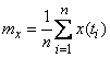In particular, with a sufficiently large expected value can be approximately calculated by the formula

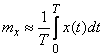. (17.8.1)

Similarly, the correlation function can be approximately found. at any . Indeed, the correlation function, by definition, is nothing more than the expectation of a random function :

(17.8.2)

This expectation can also, obviously, be approximately calculated as a time average.

We fix some value and calculate in this way the correlation function . For this, it is convenient to pre-center this implementation. , i.e., subtract the expectation from it (17.8.1):

. (17.8.3)

Calculate for a given expectation of a random function as time average. In this case, obviously, we will have to take into account not the whole time interval from 0 to , and somewhat smaller, since the second factor we are not known for everyone , but only for those for whom .

Calculating the time average of the above method, we get:

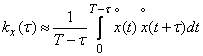. (17.8.4)

By calculating the integral (17.8.4) for a number of values , you can approximately reproduce point by point the entire course of the correlation function.

In practice, the integrals (17.8.1) and (17.8.4) are usually replaced by finite sums. We show how this is done. We divide the recording interval of a random function into equal parts long and denote the midpoints of the obtained sections (fig. 17.8.1).

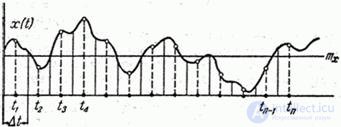
Fig. 17.8.1.

Provide integral (17.8.1) as the sum of integrals over elementary parts and on each of them we will carry out the function from the integral sign, the average value corresponding to the center of the interval . We get approximately:

,

or

. (17.8.5)

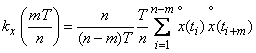
Similarly, you can calculate the correlation function for the values equal . We give, for example, the value value

calculate the integral (17.8.4), dividing the integration interval

on equal length plots and putting on each of them a function over the integral sign of the mean value. We get:

,

or finally

. (17.8.6)

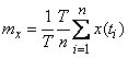
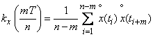
The calculation of the correlation function by the formula (17.8.6) is performed for consistently down to such values at which the correlation function becomes almost zero or starts to make small irregular fluctuations around zero. The general course of the function reproduced by individual points (Fig. 17.8.2).

Fig. 17.8.2.

In order to expectation and correlation function were determined with satisfactory accuracy, it is necessary that the number of points was large enough (about a hundred, and in some cases even a few hundred). The choice of the length of the elementary area determined by the nature of the change of the random function. If the random function changes relatively smoothly, the plot You can choose more than when it makes a sharp and frequent fluctuations. The higher-frequency composition have oscillations that form a random function, the more often it is necessary to position the reference points during processing. Approximately we can recommend to choose an elementary area so that for the full period of the highest-frequency harmonic in the composition of the random function there were about 5-10 reference points.

Often the choice of reference points does not depend on the processing at all, but is dictated by the pace of the recording equipment. In this case, it is necessary to conduct processing directly obtained from the experience of the material, not trying to insert intermediate values ​​between the observed values, since the echo can not improve the accuracy of the result, and unnecessarily complicate the processing.

Example. In the conditions of horizontal flight of the aircraft, a vertical overload acting on the aircraft was recorded. Overload was recorded at a time interval of 200 seconds with an interval of 2 seconds. The results are shown in table 17.8.1.

Table 17.8.1

Considering the process of changing overload stationary, to determine the approximate expectation of overload variance and normalized correlation function . Approximate any analytical function, find and build the spectral density of a random process.

Decision. By the formula (17.8.5) we have:

.

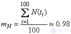We center the random function (Table 17.8.2).

Table 17.8.2

Squaring all values and dividing the amount by we obtain approximately the variance of the random function :

and standard deviation:

.

Multiplying values separated by an interval and dividing the sum of the works respectively ; ; ; ..., we obtain the values ​​of the correlation function . Normalizing the correlation function by dividing by get the table of function values (tab. 17.8.3).

Table 17.8.3

Function graph presented in fig. 17.8.3 in the form of points connected by a dotted line.

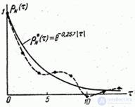
Fig. 17.8.3.

The not quite smooth course of the correlation function can be explained by the insufficient amount of experimental data (insufficient experience duration), and therefore random irregularities in the course of the function do not have time to smooth out. Calculation continued to such values ​​at which the actual correlation disappears.

In order to smooth clearly the irregular oscillations of the experimentally found function , we replace it approximately with a view function:

,

where is the parameter we select the method of least squares (see 14.5).

Using this method, we find . Calculating function values at Let's build a graph of a smoothing curve. In fig. 17.8.3 he held a solid line. The last column of the table 17.8.3 shows the values ​​of the function. .

Using the approximate expression of the correlation function (17.8.6), we obtain (see 17.4, example 1) the normalized spectral density of a random process in the form:

.

The graph of the normalized spectral density is presented in Fig. 17.8.4.

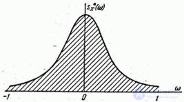
Fig. 17.8.4.