Lecture
By constructing the spectral decomposition of a stationary random function  on the final time segment
  , we obtained the spectrum of variances of a random function in the form of a series of separate discrete lines, separated by equal intervals (the so-called "discontinuous" or "ruled" spectrum).
Obviously, the more time we consider, the more complete will be our information about the random function. It is therefore natural in the spectral decomposition to try to go to the limit at  and see what happens to the spectrum of a random function. With
 ; so the distances between frequencies
  on which the spectrum is built, will be at
  unlimited decrease. In this case, the discrete spectrum will approach a continuous one, in which each arbitrarily small frequency interval
  will match the elementary variance
  .
.
Let's try to draw a continuous spectrum graphically. To do this, we must somewhat rearrange the graph of the discrete spectrum at a finite  . Namely, we will postpone the ordinate no longer the variance
  (which decreases infinitely with
  ), and the mean density of dispersion, i.e., the dispersion per unit length of a given frequency interval. Denote the distance between adjacent frequencies.
  :
:

and at each segment  as on the base, we construct a rectangle with an area
  (fig. 17.3.1). We obtain a step diagram that resembles a histogram of a statistical distribution on the basis of its construction.
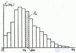
Fig. 17.3.1.
Chart height on the plot  adjacent to the point
  equal to
 (17.3.1)
and represents the average dispersion density in this region.
The total area of the whole diagram is obviously equal to the variance of the random function.
We will indefinitely increase the interval  . Wherein
  and the stepped curve will approach the smooth curve indefinitely
  (fig. 17.3.2). This curve depicts the dispersion density of the continuous spectrum frequencies, and the function itself
  called the spectral density of the dispersion, or, in short, the spectral density of the stationary random function
  .
.
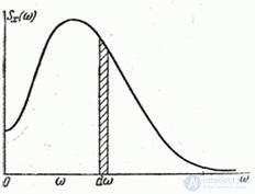
Fig. 17.3.2.
Obviously, the area bounded by the curve  , must still be equal to the variance
  random function
  :
:
 . (17.3.2)
Formula (17.3.2) is nothing more than decomposition of the variance.  for the sum of elementary terms
  , each of which is a dispersion per elementary frequency band
  adjacent to the point
  (fig. 17.3.2).
Thus, we have introduced a new additional characteristic of a stationary random process - the spectral density, which describes the frequency composition of the stationary process. However, this characteristic is not independent; it is completely determined by the correlation function of this process. Just as the ordinates of the discrete spectrum  expressed by formulas (17.2.4) through the correlation function
  spectral density
  can also be expressed through the correlation function.
We derive this expression. To do this, we proceed in the canonical expansion of the correlation function to the limit at  and see what it turns into. We will proceed from the decomposition (17.2.1) of the correlation function in a Fourier series on a finite interval
  :
:
 , (17.3.3)
where is the variance corresponding to the frequency  expressed by the formula
 . (17.3.4)
Before moving to the limit at  Let us turn to the formula (17.3.3) from the variance
  to average dispersion density
  . Since this density is calculated even at a finite value
  and depends on
  , we denote it:
 . (17.3.5)
Divide expression (17.3.4) by  ; we will receive:
 . (17.3.6)
From (17.3.5) it follows that
 . (17.3.7)
Substitute the expression (17.3.7) into the formula (17.3.3); we will receive:
 . (17.3.8)
Let's see what expression (17.3.8) will turn into  . Obviously, while
  ; discrete argument
  turns into a continuously changing argument
  ; the sum goes to the integral of the variable
  ; average dispersion density
  tends to dispersion density
  , and the expression (17.3.8) in the limit takes the form:
 , (17.3.9)
Where  - spectral density of a stationary random function.
Going to the limit at  in the formula (17.3.6), we obtain the expression of the spectral density through the correlation function:
 . (17.3.10)
An expression of the type (17.3.9) is known in mathematics as the Fourier integral. The Fourier integral is a generalization of the expansion in a Fourier series for the case of a non-periodic function considered on an infinite interval, and is a decomposition of a function into a sum of elementary harmonic oscillations with a continuous spectrum.
Just as the Fourier series expresses a decomposable function in terms of the coefficients of the series, which in turn are expressed in terms of the decomposable function, formulas (17.3.9) and (17.3.10) express functions  and
and  mutually: one over the other. The formula (17.3.9) expresses the correlation function in terms of spectral density; the formula (17.3.10), on the contrary, expresses the spectral density through the correlation function. Formulas of type (17.3.9) and (17.3.10) connecting mutually two functions are called Fourier transforms.
Thus, the correlation function and spectral density are expressed one through the other using Fourier transforms.
Note that from the general formula (17.3.9) with  we obtain the previously obtained decomposition in frequency (17.3.2).
In practice, instead of spectral density  often use the normalized spectral density:
 , (17.3.11)
Where  - variance of a random function.
It is easy to verify that the normalized correlation function  and normalized spectral density
  connected by the same Fourier transforms:
 (03/17/12)
Assuming in the first of equalities (17.3.12)  and considering that
  , we have:
 , (17.3.13)
that is, the total area bounded by the graph of the normalized spectral density is equal to one.
Example 1. Normalized correlation function  random function
  linearly decreasing from one to zero with
  ; at
; at 
 (fig. 17.3.3).
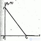
Fig. 17.3.3.
Determine the normalized spectral density of a random function  .
.
Decision. The normalized correlation function is expressed by the formulas:

From the formulas (17.3.12) we have:
 .
.
The graph of the normalized spectral density is presented in Fig. 17.3.4.
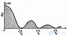
Fig. 17.3.4.
The first - the absolute - maximum spectral density is reached at  ; By disclosing uncertainty at this point, make sure that it is equal to
  . Further, with increasing
  spectral density reaches a number of relative maxima, whose height decreases with increasing
  at
at 
 .
.
The nature of the change in spectral density  (fast or slow decay) depends on the parameter
  . Full area bounded by the curve
  , is constant and equal to one. Change
  tantamount to changing the scale of the curve
  on both axes while maintaining its area. By increasing
  the scale on the ordinate axis increases, on the abscissa axis - decreases; the predominance of zero frequency in the spectrum of a random function becomes more pronounced. In the limit at
  the random function degenerates into a normal random variable; wherein
  and the spectrum becomes discrete with a single frequency
  .
.
Example 2. Normalized spectral density  random function
  constant over a certain frequency range
  and is equal to zero outside this interval (fig. 17.3.5).
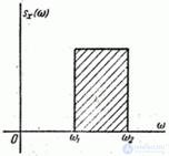
Fig. 17.3.5.
Determine the normalized correlation function of a random function  .
.
Decision. Value  at
at  determined from the condition that the area bounded by the curve
  , is equal to one:
 ,
,  .
.
From (17.3.12) we have:

 .
.
General view of the function  shown in fig. 17.3.6.
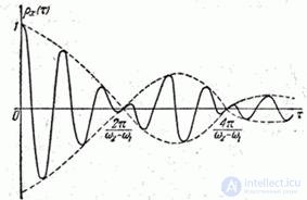
Fig. 17.3.6.
It has the character of oscillations decreasing in amplitude with a number of nodes at which the function vanishes. The specific type of graph obviously depends on the values  .
.
Of interest is the limiting view of the function.  at
at  . Obviously when
  the spectrum of a random function is discrete with a single line corresponding to the frequency
  ; at the same time, the correlation function turns into a simple cosine wave:
 .
.
Let's see what kind of random function itself has in this case.  . With a discrete spectrum with a single line, the spectral decomposition of a stationary random function
  has the form:
 , (17.3.14)
Where  and
and  - uncorrelated random variables with a mathematical expectation of zero and equal variances:
 .
.
Let us show that a random function of the type (17.3.14) can be represented as one harmonic oscillation frequency  with random amplitude and random phase. Denoting
 ,
,  ,
,
we bring the expression (17.3.14) to the form:
 .
.
In this expression  , the random amplitude;
  - random phase of harmonic oscillation.
So far, we have considered only the case when the distribution of dispersions in frequencies is continuous, that is, when an infinitesimally small dispersion falls on an infinitesimal portion of frequencies. In practice, sometimes there are cases when a random function has in its composition a purely periodic frequency component  with a random amplitude. Then, in the spectral decomposition of a random function, in addition to the continuous spectrum of frequencies, there will also be a separate frequency
  with a finite variance
 .In general, there may be several such periodic components. Then the spectral decomposition of the correlation function will consist of two parts: the discrete and continuous spectrum:
 . (03/17/15)
Cases of stationary random functions with such a “mixed” spectrum are rather rare in practice. In these cases, it always makes sense to divide the random function into two terms — with a continuous and discrete spectrum — and examine these terms separately.
Relatively often we have to deal with a special case when the final dispersion in the spectral decomposition of a random function falls at zero frequency (  ). This means that a random variable with variance is included as part of the random function.
  . In such cases, it also makes sense to select this random term and operate with it separately.
Comments
To leave a comment
Probability theory. Mathematical Statistics and Stochastic Analysis
Terms: Probability theory. Mathematical Statistics and Stochastic Analysis