Lecture
Consider some stationary random function.  and suppose you want to evaluate its characteristics: expectation
  and correlation function
  . Above (see
  15.4) ways to obtain these characteristics from experience were outlined. For this you need to have a known number of implementations of a random function.
  . By processing these implementations, one can find estimates for the expectation
  and correlation function
  . Due to the limited number of observations (function
  will not be strictly constant; it will have to be averaged and replaced by some constant
  ; similarly, averaged values
  for different
  , we obtain the correlation function
  .
.
This processing method is obviously quite complicated and cumbersome, and also consists of two stages: an approximate determination of the characteristics of a random function and also an approximate averaging of these characteristics. Naturally, the question arises: is it possible for a stationary random function to replace this complex, two-step process with a simpler one, which is based in advance on the assumption that the expectation does not depend on time, and the correlation function on the origin?
In addition, the question arises: when processing observations of a stationary random function, is it essential to have several realizations? Since the random process is stationary and proceeds uniformly in time, it is natural to assume that a single realization of sufficient duration can serve as sufficient experimental material for obtaining the characteristics of a random function.
Looking more closely at this issue, it turns out that such a possibility does not exist for all random processes: it is not always that a single implementation of sufficient duration turns out to be equivalent to a set of individual realizations.
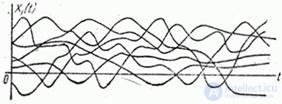
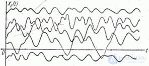
For example, consider two stationary random functions.  and
and  , presented by set of the implementations on fig. 17.7.1 and 17.7.2.

Fig. 17.7.1.

Fig. 17.7.2.
For random function  The following peculiarity is characteristic: each of its realizations has the same characteristic features: the average value around which oscillations occur, and the average span of these oscillations. Let us randomly choose one of such realizations and continue the mental experience, as a result of which it was obtained, for a certain period of time.
  . Obviously, with a sufficiently large
  this one implementation can give us a fairly good idea of the properties of the random function as a whole. In particular, the average value of this implementation along the abscissa axis - over time, we must obtain an approximate value of the expectation of a random function; averaging the squares of deviations from this mean, we should get an approximate value of the variance, and so on.
They say that such a random function has an ergodic property. The ergodic property is that each individual implementation of a random function is, as it were, an “authorized representative” of the entire set of possible realizations; one implementation of sufficient duration can replace when processing multiple implementations of the same total duration.
Consider now a random function.  . Choose arbitrarily one of its implementations, continue it mentally for a sufficiently large portion of time, and calculate its average value over time throughout the entire observation segment. Obviously, this average value for each implementation will be its own and may differ significantly from the mathematical expectation of a random function constructed as an average of many implementations. It is said about such a random function that it does not possess an ergodic property.
If random function  possesses an ergodic property, then for it the average in time (on a sufficiently large observation area) is approximately equal to the average in many observations. The same will be true for
  ,
,  and so on. Therefore, all the characteristics of a random function (expectation, variance, correlation function) can be approximately determined by one sufficiently long implementation.
Which stationary random functions have, and which do not have ergodic properties?
We will clarify this question clearly, based on an example. Consider a random function  - fluctuations of the angle of attack of the aircraft in steady state horizontal flight. Suppose that the approach occurs in some typical average meteorological conditions. Oscillations of the angle of attack are caused by random disturbances associated with the turbulence of the atmosphere. The average value of the angle of attack around which oscillations occur depends on the altitude
  . It depends on this height and the range of oscillations: it is known that in the lower layers of the atmosphere, turbulence is stronger than in the upper layers.
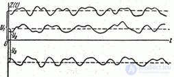
Consider a random function  - fluctuations of the angle of attack at a given height
  . Each of the implementations of this random function is carried out as a result of exposure to the same group of random factors and has the same probabilistic characteristics; random function
  possesses ergodic properties (fig. 17.7.3).

Fig. 17.7.3.
Imagine now that a random function is considered.  not for one height
  , and for the whole range within which some law of height distribution is set (for example, the law of uniform density). Such a random function, while remaining stationary, obviously, will no longer have an ergodic property; its possible implementations, carried out with some probabilities, have a different character (Fig. 17.7.4).

Fig. 17.7.4.
This random process is characterized by the fact that it is sort of “decomposed” into more elementary random processes; Each of them is carried out with a certain probability and has its own individual characteristics. Thus, the decomposability, the internal heterogeneity of a random process occurring with some probability in one way or another, is the physical cause of the non-ergodicity of this process.
In particular, the nonergodicity of a random process can be related to the presence in its composition of a term as an ordinary random variable (i.e., the presence in the spectrum of a random process, in addition to the continuous part, of a finite dispersion at a frequency of 0).
Indeed, consider the random function
 , (17.7.1)
Where  - ergodic stationary random function with characteristics
  ,
,  ;
;  - random variable with characteristics
  and
and  ; suppose moreover that
  and
and  uncorrelated.
Define the characteristics of a random function  . According to the general rules of addition of random functions (see
  15.8) we have:
 , (17.7.2)
 . (17.7.3)
It can be seen from formulas (17.7.2) and (17.7.3) that the random function  is stationary. But does it have ergodic properties? Obviously not. Each of its implementation will differ in character from the others, will have one or another time average value depending on what value the random variable has taken.
  (fig. 17.7.5).

Fig. 17.7.5.
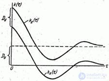
The ergodicity or nonergodicity of a random process can be directly indicated by the form of its correlation function. Indeed, consider the correlation function of the non-ergodic random function (17.7.1). It differs from the correlation function of the random function.  the presence of a constant term
  (fig. 17.7.6).

Fig. 17.7.6.
While the correlation function  tends to zero at
  (the correlation between the values of a random function decreases unlimitedly as the distance between them increases), the function
  no longer tends to zero at
  , and is approaching a constant value
  .
.
In practice, we do not have the opportunity to investigate a random process and its correlation function over an infinite segment of time; value range  that we deal with is always limited. If at the same time the correlation function of the stationary random process with increasing
  not decreasing, and starting from some
  , remains approximately constant, this is usually a sign that the composition of a random function has a summand in the form of an ordinary random variable and that the process is not ergodic. The tendency of the correlation function to zero at
  speaks in favor of the ergodicity of the process. In any case, it is sufficient for the expectation of a function to be defined as the average over time.
When solving practical problems, the ergodicity of a random process is often made not on the basis of a study of the behavior of the correlation function when  , and on the basis of physical considerations related to the essence of the process (its supposed “decomposability” or “indecomposability” into elementary processes of various types that appear with certain probabilities).
Comments
To leave a comment
Probability theory. Mathematical Statistics and Stochastic Analysis
Terms: Probability theory. Mathematical Statistics and Stochastic Analysis