14.4. Exact methods for constructing confidence intervals for random variable parameters

Exact methods for constructing confidence intervals for parameters of a random variable distributed according to the normal law

In the previous We considered roughly approximate methods for constructing confidence intervals for expectation and variance. In this we will give an idea of ​​the exact methods of solving the same problem. We emphasize that to accurately determine the confidence intervals, it is absolutely necessary to know in advance the form of the distribution law whereas it is not necessary for the application of approximate methods.

The idea of ​​accurate methods for constructing confidence intervals is as follows. Any confidence interval is found from a condition expressing the probability of certain inequalities that include the estimate we are interested in. . Distribution law in general, depends on the unknown parameters themselves . However, sometimes it is possible to move in inequalities from a random variable to some other function of the observed values , the distribution law of which does not depend on unknown parameters, but depends only on the number of experiments and on the type of distribution law . Such random variables play a large role in mathematical statistics; they are most studied in the case of a normal distribution of magnitude .

For example, it is proved that with a normal distribution of random value

, (14.4.1)

Where

, ,

obeys the so-called student distribution law with degrees of freedom; the density of this law is

(14.4.2)

Where - known gamma function:

.

It is also proved that the random variable

(14.4.3)

has a "distribution " with degrees of freedom (see Ch. 7. p. 145), the density of which is expressed by the formula

(14.4.4)

Without dwelling on the conclusions of the distributions (14.4.2) and (14.4.4), we will show how they can be applied when building confidence intervals for the parameters and .

Let produced independent experiments on a random variable distributed according to normal law with unknown parameters and . Estimates for these parameters

, .

It is required to build confidence intervals for both parameters corresponding to the confidence probability. .

We first construct the confidence interval for the expectation. Naturally, this interval is symmetric with respect to ; denote half the length of the interval. Magnitude need to choose so that the condition is met

. (14.4.5)

Let's try to go to the left side of equality (14.4.5) from the random variable to a random value distributed by the law of student. To do this, multiply both sides of the inequality by a positive value :

or, using the designation (14.4.1),

. (14.4.6)

Find such a number , what

. (14.4.7)

Magnitude there is a condition

. (14.4.8)

From the formula (14.4.2) it is clear that - even function; therefore (14.4.8) gives

. (14.4.9)

Equality (14.4.9) determines the value depending on the . If you have at your disposal a table of values ​​of the integral

,

This value can be found by reverse interpolation in this table. However, it is more convenient to make a table of values ​​in advance. . Such a table is given in the annex (see Table 5). This table shows the values depending on confidence probability and numbers of degrees of freedom . Defining according to table 5 and believing

(14.4.10)

we will find half the width of the confidence interval and the interval itself

. (14.4.11)

Example 1. Produced 5 independent experiments on a random variable distributed normally with unknown parameters and . The results of the experiments are given in table 14.4.1.

Table 14.4.1

Find a rating for the expectation and build for it a 90% confidence interval (i.e., the interval corresponding to the confidence probability ).

Decision. We have

; .

According to table 5 of the application for and we find

,

from where

.

Confidence interval will be

.

Example 2. For the conditions of example 1 14.3, assuming the value distributed normally, find the exact confidence interval.

Decision. According to table 5 of the application we find when and

; from here .

Comparing with the solution of example 1 14.3 ( ), we are convinced that the discrepancy is very slight. If we keep the accuracy up to the second decimal place, then the confidence intervals found by the exact and approximate methods are the same:

.

Let us proceed to the construction of a confidence interval for variance.

Consider the unbiased variance estimate.

and express the random variable in terms of (14.4.3), having a distribution (14.4.4):

. (14.4.12)

Knowing the law of distribution of magnitude , you can find the interval with which it falls with a given probability .

Distribution law magnitudes has the form shown in fig. 14.4.1.

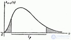
Fig. 14.4.1.

The question arises: how to choose the interval ? If the distribution law was symmetrical (like a normal law or student’s t-distribution), it would be natural to take the interval symmetric with respect to the expectation. In this case, the law asymmetrical We agree to choose an interval so that the probability of the output value outside the interval to the right and left (the shaded areas in Fig. 14.4.1) were the same and equal

.

To build an interval with this property, we use table 4 of the appendix: it shows the numbers such that

for size having distribution with degrees of freedom. In our case . Fix and find in the corresponding row table. 4 two values ; one that corresponds to probability , other - probabilities . Denote these values and . Interval It has to your left as well - right end.

Now we find by interval sought confidence interval for dispersion with borders and that covers the point with probability :

.

We construct such an interval that covers a point if and only if the value falls within the interval . We show that the interval

(14.4.13)

satisfies this condition. Indeed, inequalities

;

equal inequalities

; ,

and these inequalities are fulfilled with probability . Thus, the confidence interval for the dispersion is found and expressed by the formula (14.4.13).

Example 3. Find the confidence interval for the variance under the conditions of Example 2 14.3 if it is known that the value is distributed normally.

Decision. We have ; ; . According to table 4 of the application we find when

for ;

for .

According to the formula (14.4.13) we find the confidence interval for the variance

.

The corresponding interval for the standard deviation: . This interval only slightly exceeds that obtained in example 2 14.3 approximate spacing method .