Lecture
In some practical tasks, there are continuously random variables, which are known in advance that their possible values lie within a certain defined interval; in addition, it is known that within this interval, all values of a random variable are equally likely (more precisely, they have the same probability distribution density). Such random variables are said to be distributed according to the law of uniform density.
We give several examples of such random variables.
Example 1. The body was weighed on an accurate scale, but at the weighing body there are only weights weighing at least 1g; the weighing result indicates that the body weight is between  and
and  grams. Body weight is assumed equal
  grams The mistake made at the same time
  obviously there is a random variable distributed with a uniform density on the plot
  year
year
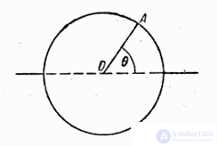
Example 2. A vertical symmetrical wheel (fig. 5.8.1) is rotated and then stopped due to friction. Considered a random variable  - the angle that, after stopping, will be with the horizon a fixed radius of the wheel OA. Obviously the magnitude
  distributed with uniform density on the plot
  .
.

Fig. 5.8.1.
Example 3. Metro trains run at intervals of 2 minutes. The passenger goes to the platform at some point in time. The time T, during which he will have to wait for the train, is a random variable distributed with a uniform density over a stretch of (0.2) minutes.

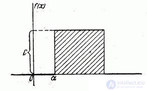
Fig. 5.8.2.
Consider a random variable  subordinate to the law of uniform density in the area from
  before
  (fig. 5.8.2), and we write for it an expression of the distribution density
  . Density
  is constant and equal to c on the segment
  ; outside this segment, it is zero:

Since the area bounded by the distribution curve is one:

that

and distribution density  has the form:
 (5.8.1)
Formula (5.8.1) and expresses the law of uniform density on the site  .
.
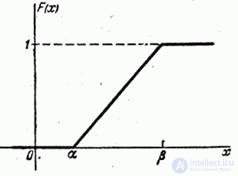
We write an expression for the distribution function  . The distribution function is expressed by the area of the distribution curve to the left of the point.
  . Consequently,

Function graph  is shown in fig. 5.8.3.

Fig. 5.8.3.
Define the basic numerical characteristics of a random variable.  subordinate to the law of uniform density in the area from
  before
  .
.
Expectation value X:
 (5.8.2)
Due to the symmetry of the uniform distribution, the median of  also equal to
  .
.
Fashion law of uniformity of density is not.
According to the formula (5.7.16) we find the variance of the value  :
:
 (5.8.3)
where the standard deviation
 (5.8.4)
Due to the symmetry of the distribution, its asymmetry is zero:
 . (5.8.5)
To determine the excess, we find the fourth central point:

from where
 (5.8.6)
Determine the average arithmetic deviation:
 (5.8.7)
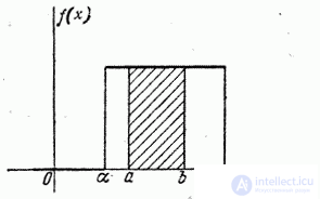
Finally, we find the probability of hitting a random variable.  distributed according to the law of uniform density on the plot
  representing part of a plot
  (fig. 5.8.4). Geometrically, this probability is the area shaded in Fig. 5.8.4. Obviously, it is equal to:
 (5.8.8)
those. the ratio of the length of the segment  to the entire length of the section
  on which uniform distribution is set.

Fig. 5.8.4.
Comments
To leave a comment
Probability theory. Mathematical Statistics and Stochastic Analysis
Terms: Probability theory. Mathematical Statistics and Stochastic Analysis