Galton's board (quincunks) to demonstrate the central limit theorem

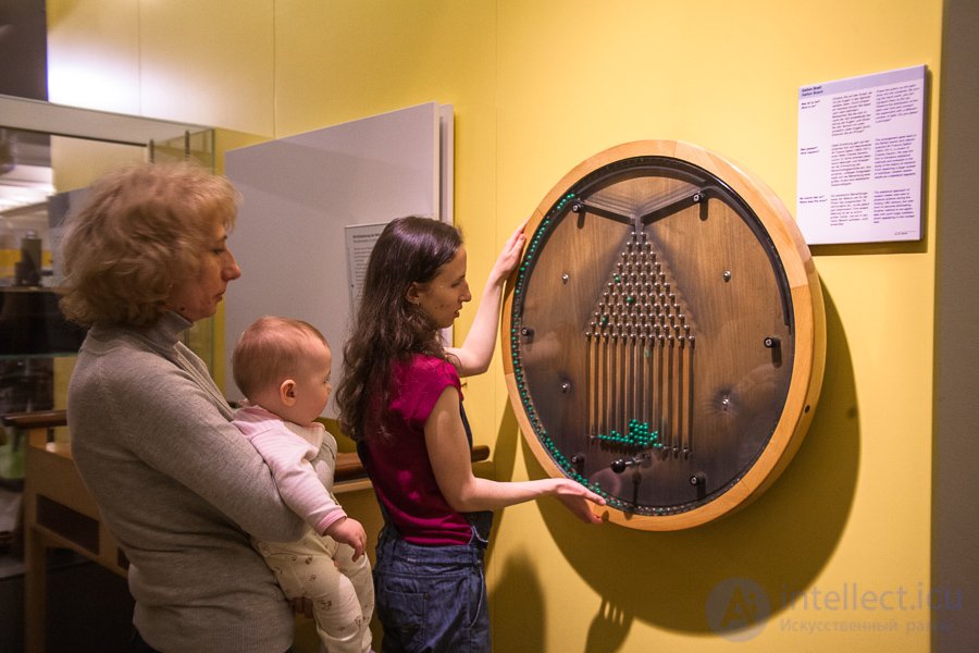
Galton Board (English Galton box , also common names quincunks , quincunx and bean machine ) - a device invented by the English scientist Francis Galton (the first copy was made in 1873 ^[1] , then the device was described by Galton in the book Natural inheritance , published in 1889 year) and intended to demonstrate the central limit theorem.

Device board

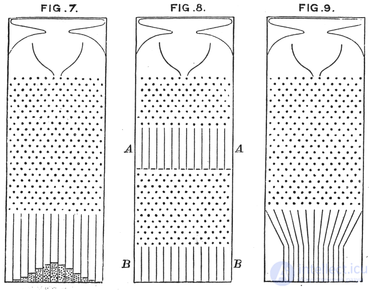
Galton's board is a box with a transparent front wall. Pins that form a triangle are hammered into the back wall. From the top, balls are thrown into the box through the funnel (the exit from which is located exactly midway between the left and right walls). In the ideal case, when colliding with a pin, the ball with the same probability can turn either to the right or to the left. The lower part of the box is divided by partitions (the number of which is equal to the number of pins in the bottom row), as a result of which the balls, rolling down to the bottom of the box, form bars, which are the higher, the closer to the middle of the board (with a sufficiently large number of balls, the bars look like normal distribution).

If you draw Pascal's triangle on the back wall, you can see how many ways you can get to each of the pins (the closer the pin to the center, the greater the number of ways).

Some board games, as well as the Patinko slot machine, use a Galton board or devices similar to it.

Ball distribution

Denote as n the total number of collisions of the ball with pins; as k is the number of times when the ball turns to the right (thus, it appears in the k- th column in order). Then the number of ways in which it can reach the kth column is determined by the binomial coefficient . It follows that the probability of being in the kth column is equal to where p is the probability of turning to the right (usually we can assume that ). This is the probability function of the nominal distribution, which, in accordance with the central limit theorem for a sufficiently large n, approximates the normal distribution.

Calculation example

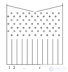
Galton's board is a box, on the back wall of which two inclined planks are reinforced, forming a funnel; in the middle - several rows of nails hammered into the wall and staggered; below - a system of identical vertical cells (Fig. 1.1). The front wall of the box is glass.

We number the cells 1, 2, ..., . Take a pea, throw it in the funnel and follow its movement. A pea, having undergone a series of collisions with nails, will fall into some, for example, i -th cell. We will get a pea from the box and again throw it in the funnel. And now the pea after a series of collisions with nails falls into some cell. But in general, this cell will be different. Let us make so N throws of a pea, each time noting which cell it falls into. Let n ₁ be the number of hits in the first cell, n ₂ in the second, etc., n _i in the i -th one, n _k in the k -th one. The number N is called the number of trials, and the number the number of positive outcomes. Attitude - the frequency of positive outcomes for the i -th cell.

If N is large (ideally infinitely large), then - probability of a positive outcome, i.e. probability that a pea after a collision with nails falls into the i -th cell.

In all these considerations it is very important to note the following:

1. Pea collisions with nails are random (unpredictable) processes. We never know which nails, how many nails and how the pea will collide.
2. Since the collisions are random, we never know where and at what speed the pea leaves the layer of nails and, as a result, which cell it enters.

The trajectory of the pea, the number of collisions, the final speed (after the last collision), the cell into which the pea falls are all a matter of chance, while the number of shots (trials) is small. Although the movement of the pea obeys the laws of mechanics of Galileo-Newton, we cannot know the final result. Another thing, when the number of tests (throws) is huge. The trajectory and the number of collisions of the pea are also unpredictable, but we can calculate the final speed and the number of hits in the i -th cell with some probability. We construct a histogram of frequencies of positive outcomes and draw an envelope. In the case when , each of the bars of the histogram corresponds to the probability of a positive outcome, then .

But P _i is the area of ​​the i -th bar on the histogram and - area under the envelope curve (Fig. 1.2).

The envelope curve shows how the probabilities are distributed by cell number. The mathematical function to which this curve corresponds is called the statistical probability distribution function. In our particular case, this statistical distribution is called normal, and the function is called the Gauss function. Its analytical expression is:

where P _i is the probability of the i -th positive outcome, n _i is the number of positive i -th outcomes, C is some constant, e, is the base of the natural logarithm, - expectation, which is as
where N is the number of tests.

Change the nature of the experience. Take N identical peas and throw each of them into the funnel once. We have the right to expect the result already obtained. Why? Peas are exactly the same! Consequently, the result will be the same.

Change the nature of the experience again. Take N identical peas and pour them all at once into the funnel. What will change in the movement of peas? The number of collisions will change, because Now the peas are faced not only with nails, but also with each other. But in the final case, all the peas are distributed into cells. Denote - the number of peas in the i- th cell, then - the probability that the pea will fall into the i -th cell. Paying attention to the fact that the probability distribution curve has the same character as in the two previous experiments, we come to the conclusion:

those. our system of N peas obeys the statistical law of distribution. The final conclusion: a system of N elements with internal random processes obeys the laws of statistics. Such systems are called statistical systems.