Lecture
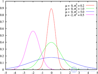
Probability density The green line corresponds to the standard normal distribution. |
|
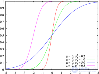
Distribution function The colors on this graphic correspond to the graphic above. |
|
| Designation |  |
| Options | μ - shift coefficient (real number) σ > 0 - scale factor (real, strictly positive) |
| Carrier |  |
| Probability density |  |
| Distribution function |  |
| Expected value |  |
| Median |  |
| Fashion |  |
| Dispersion |  |
| Asymmetry coefficient |  |
| Coefficient of kurtosis |  |
| Informational entropy |  |
| Generating function of moments |  |
| Characteristic function |  |
The normal distribution , [1] [2] also referred to as the Gauss distribution, is the probability distribution, which in the one-dimensional case is given by a probability density function, the same Gauss function:

where the parameter μ is the mean (average), the median and the mode of distribution, and the parameter σ is the standard deviation ( σ ² - dispersion) of the distribution.
Thus, the one-dimensional normal distribution is a two-parameter family of distributions. The multidimensional case is described in the article “Multidimensional Normal Distribution”.
The standard normal distribution is called the normal distribution with the expectation μ = 0 and the standard deviation σ = 1.
The importance of the normal distribution in many areas of science (for example, in mathematical statistics and statistical physics) follows from the central limit theorem of probability theory. If the observation result is the sum of many random weakly interdependent quantities, each of which makes a small contribution relative to the total sum, then with an increase in the number of terms, the distribution of the centered and normalized result tends to normal. This law of probability theory has the consequence of a wide distribution of the normal distribution, which was one of the reasons for its name.
Moments and absolute moments of a random variable X are called the expectation X p and  , respectively. If the expectation of the random variable μ = 0, then these parameters are called central moments . In most cases, moments for p are of interest.
If X has a normal distribution, then for it there exist (finite) moments for all p with a real part greater than −1. For nonnegative integer p , the central moments are as follows:

Here n is a positive integer, and the record ( p - 1) !! means a double factorial of the number p - 1, that is (since p - 1 is odd in this case) the product of all odd numbers from 1 to p - 1.
The central absolute moments for non-negative integers p are as follows:

The last formula is also valid for arbitrary p > −1.
The normal distribution is infinitely divisible.
If random values  and
and  independent and have a normal distribution with mathematical expectations
  and
and  and dispersions
  and
and  accordingly,
  also has a normal distribution with the expectation
  and variance
  It follows that a normal random variable is representable as the sum of an arbitrary number of independent normal random variables.
The normal distribution is a continuous distribution with maximum entropy for a given expectation and variance [3] [4] .
The simplest approximate modeling methods are based on the central limit theorem. Namely, if we add up several independent equally distributed quantities with a finite variance, then the sum will be distributed approximately normally. For example, if we add 100 independent standard uniformly distributed random variables, then the distribution of the sum will be approximately standard normal .
For software generation of normally distributed pseudo-random variables, it is preferable to use the Box-Muller transform. It allows you to generate one normally distributed value on the basis of one evenly distributed.
Normal distribution is often found in nature. For example, the following random variables are well modeled by a normal distribution:
Such a wide distribution of this distribution is due to the fact that it is an infinitely divisible continuous distribution with finite variance. Therefore, some others, such as the binomial and Poisson, approach it in the limit. This distribution simulates many non-deterministic physical processes. [five]
The multidimensional normal distribution is used in the study of multidimensional random variables (random vectors). One of the many examples of such applications is the study of the properties of a person’s personality in psychology and psychiatry.
Comments
To leave a comment
Probability theory. Mathematical Statistics and Stochastic Analysis
Terms: Probability theory. Mathematical Statistics and Stochastic Analysis