Lecture
In Chapter 5, we introduced into consideration the numerical characteristics of a single random variable.  - the initial and central moments of different orders. Of these characteristics, the most important are two: the expectation
  and variance
  .
.
Similar numerical characteristics — the initial and central moments of different orders — can also be introduced for a system of two random variables.
Initial moment of order  ,
,  systems
  called the expectation of the work
  on
on  :
:
 . (8.6.1)
Central point of order  systems
  called the expectation of the work
  th and
  th degree corresponding centered values:
 , (8.6.2)
Where  ,
,  .
.
We write out the formulas that serve to directly count the moments. For discontinuous random variables
 , (8.6.3)
 , (8.6.4)
Where  - the probability that the system
  will take values
  , and summation is spread over all possible values of random variables.
  ,
,  .
.
For continuous random variables:
 , (8.6.5)
 , (8.6.6)
Where  - the distribution density of the system.
Besides  and
and  characterizing the moment order with respect to individual quantities, the total moment order is also considered
  equal to the sum of the exponents at
  and
and  . According to the total order, the moments are classified into first, second, etc. In practice, only the first and second moments are usually used.
The first initial moments are already known to us the expected values of  and
and  Included in the system:

Set of mathematical expectations  is a characteristic of the position of the system. Geometrically, these are the coordinates of the midpoint on the plane around which the point is scattered.
  .
.
Besides the first initial moments, the second central moments of the system are widely used in practice. Two of them are already known variances of quantities  and
and  :
:

characterizing the dispersion of a random point in the direction of the axes  and
and  .
.
The second mixed central moment plays a special role as a characteristic of the system:
 ,
,
those. expectation of product of centered quantities.
In view of the fact that this moment plays an important role in the theory, we introduce a special designation for it:
 . (8.6.7)
Characteristic  is called the correlation moment (otherwise - “moment of connection”) of random variables
  ,
,  .
.
For discontinuous random variables, the correlation moment is expressed by the formula
 , (8.6.8)
and for continuous - by the formula
 . (8.6.9)
Find out the meaning and purpose of this characteristic.
Correlation moment is a characteristic of a system of random variables, describing, besides, the dispersion of quantities  and
and  , also the connection between them. In order to verify this, we prove that for independent random variables the correlation moment is zero.
The proof is carried out for continuous random variables. Let be  ,
,  - independent continuous quantities with distribution density
  . AT
. AT  8.5 we proved that for independent variables
 . (8.6.10)
Where  ,
,  - distribution density, respectively
  and
and  .
.
Substituting the expression (8.6.10) into the formula (8.6.9), we see that the integral (8.6.9) turns into a product of two integrals:
 .
.
Integral

is nothing but the first central moment of magnitude  , and, therefore, is zero; for the same reason is zero and the second factor; hence for independent random variables
  .
.
Thus, if the correlation moment of two random variables is nonzero, this is a sign of the dependence between them.
From the formula (8.6.7) it can be seen that the correlation moment characterizes not only the dependence of the quantities, but also their dispersion. Indeed, if, for example, one of the quantities  deviates very little from its expectation (almost non-random), then the correlation moment will be small, no matter how closely related the quantities are
  . Therefore, to characterize the relationship between the quantities
  pure pass from the moment
  to dimensionless characteristic
 , (8.6.11)
Where  ,
,  - standard deviations of magnitudes
  ,
,  . This characteristic is called the coefficient of correlation
  and
and  . Obviously, the correlation coefficient vanishes simultaneously with the correlation moment; therefore, for independent random variables, the correlation coefficient is zero.
Random variables for which the correlation moment (and, hence, the correlation coefficient) is equal to zero, are called uncorrelated (sometimes - “unrelated”).
Let us find out if the notion of uncorrelated random variables is equivalent to the notion of independence. We have proved above that two independent random variables are always uncorrelated. It remains to be seen: is the reverse situation true, does their independence follow from the uncorrelatedness of the values? It turns out - no. It is possible to construct examples of such random variables that are uncorrelated, but dependent. The equality to zero of the correlation coefficient is a necessary, but not sufficient condition for the independence of random variables. Independence of random variables implies their uncorrelatedness; on the contrary, their independence does not follow from the uncorrelated values. The condition of independence of random variables is more stringent than the condition of uncorrelatedness.
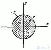
We will see this with an example. Consider a system of random variables  distributed with uniform density inside the circle
  radius
  centered at the origin (Fig. 8.6.1).

Fig.8.6.1
Distribution density  expressed by the formula

From the condition  we find
  .
.
It is easy to verify that in this example, the values are dependent. Indeed, it is immediately clear that if the magnitude  took, for example, the value 0, then the value
  can equally well take all values from
  before
  ; if the quantity
  took meaning
  then quantity
  can take only one single value, exactly zero; in general, the range of possible values
  depends on what value took
  .
.
Let's see if these values are correlated. Calculate the correlation moment. Bearing in mind that for symmetry reasons  , we get:
 . (8.6.12)
To calculate the integral, we divide the integration domain (the circle  ) into four sectors
  corresponding to the four coordinate angles. In sectors
  and
and  integrand is positive in sectors
  and
and  - negative; in their absolute value, the integrals for these sectors are equal; therefore, the integral (8.6.12) is zero, and the quantities
  not correlated.
Thus, we see that random variables do not always follow from the uncorrelatedness of random variables.
The correlation coefficient characterizes not every dependence, but only the so-called linear dependence. The linear probabilistic dependence of random variables is that as one random variable increases, the other tends to increase (or decrease) according to a linear law. This tendency towards linear dependence may be more or less pronounced, more or less approximate to functional, i.e., the closest linear dependence. The correlation coefficient characterizes the degree of closeness of the linear relationship between random variables. If random values  and
and  linked by an exact linear functional dependence:
 .
.
that  and the plus or minus sign is taken depending on whether the coefficient is positive or negative.
  . In general, when the quantities
  and
and  linked by an arbitrary probabilistic dependence, the correlation coefficient may have a value within:
 .
.
When  speak of a positive correlation of magnitudes
  and
and  , when
  - about negative correlation. A positive correlation between random variables means that as one increases, the other tends to increase on average; a negative correlation means that as one of the random variables increases, the other tends to decrease on average.
In the considered example, two random variables  distributed inside a circle with a uniform density, despite the existence of a relationship between
  and
and  , linear dependence is absent; with increasing
  only the range of change changes
  , and its mean value does not change; naturally quantities
  turn out to be uncorrelated.

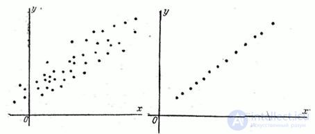
Fig. 8.6.2 Fig.8.6.3
Let us give some examples of random variables with positive and negative correlation.
1. Weight and height of a person are associated with a positive correlation.
2. The time spent on adjusting the device when preparing it for work, and the time of its trouble-free operation are associated with a positive correlation (if, of course, time is spent wisely). On the contrary, the time spent on preparation and the number of faults detected during operation of the device are associated with a negative correlation.
3. When firing a volley, the coordinates of the points of hit of individual projectiles are associated with a positive correlation (since there are common aiming errors for all shots, each deviating from the target equally).
4. Two shots are fired at the target; the point of entry of the first shot is recorded, and an amendment is introduced into the scope proportional to the error of the first shot with the opposite sign. The coordinates of the hit points of the first and second shots will be associated with a negative correlation.
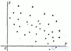
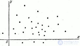
If we have at our disposal the results of a series of experiments on a system of random variables  then it is easy to judge about the presence or absence of a significant correlation between them in the first approximation according to the graph, which shows all the pairs of random values obtained from the experience as points. For example, if the observed pairs of values of values are arranged as shown in Fig. 8.6.2, this indicates the presence of a pronounced positive correlation between the quantities. An even more pronounced positive correlation, close to a linear functional dependence, is observed in Fig. 8.6.3. In fig. 8.6.4 shows a case of relatively weak negative correlation. Finally, in fig. 8.6.5 illustrates the case of practically uncorrelated random variables. In practice, before investigating the correlation of random variables, it is always useful to preliminarily construct the observed pairs of values on the graph for the first qualitative judgment on the type of correlation.


Fig. 8.6.4 Figure 8.6.5
Methods for determining the characteristics of a system of random variables from experiments will be covered in Chapter 14.
Comments
To leave a comment
Probability theory. Mathematical Statistics and Stochastic Analysis
Terms: Probability theory. Mathematical Statistics and Stochastic Analysis