Lecture
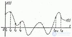
Consider some random function.  for a certain period of time (Fig. 15.2.1).

Fig. 15.2.1.
Strictly speaking, we cannot depict a random function using a curve on a graph: we can only draw its specific implementations. However, for the sake of clarity, you can allow yourself to arbitrarily draw a random function in the drawing.  in the form of a curve, meaning by this curve is not a specific implementation, but the entire set of possible implementations
  . This convention we will mark by the fact that the curve, symbolically depicting a random function, we will carry out a dotted line.
Suppose that the course of a change in a random function is registered with the help of some device that does not record a random function continuously, but marks its values at certain intervals - at times  .
.
As stated above, with a fixed value  a random function turns into a regular random variable. Consequently, the recording results in this case are a system
  random variables:
 . (15.2.1)
Obviously, at a sufficiently high rate of operation of the recording equipment, recording a random function at such intervals will give a fairly accurate idea of the course of its change. Thus, the consideration of a random function can be replaced with a certain approximation by the consideration of a system of random variables (15.2.1). As you increase  such a replacement is becoming more and more accurate. In the limit, the number of values of the argument — and accordingly the number of random variables (15.2.1) — becomes infinite. Thus, the concept of a random function can be viewed as a natural generalization of the concept of a system of random variables to the case of an infinite (uncountable) set of quantities included in the system.
Proceeding from this interpretation of a random function, let us try to answer the question: what should be the law of distribution of a random function?
We know that the law of distribution of one random variable is a function of one argument, the law of distribution of a system of two variables is a function of two arguments, etc. However, the practical use of probabilities of functions of many arguments is so inconvenient that even for systems of three or four variables we we usually refuse to use the laws of distribution and consider only numerical characteristics. As for the law of distribution of a random function, which provides a function of an innumerable set of arguments, then such a law can at best be written in a purely formal form in some symbolic form; the practical use of such a characteristic is obviously completely excluded.
It is possible, however, for a random function to construct some probability characteristics similar to the laws of distribution. The idea of building these characteristics is as follows.
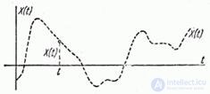
Consider a random variable  - cross section of a random function at the moment
  (fig. 15.2.2).

Fig. 15.2.2.
This random variable obviously has a distribution law, which generally depends on  . Denote it
  . Function
  called the one-dimensional distribution law of a random function
  .
.
Obviously function  not a complete, exhaustive characteristic of a random function
  . Indeed, this function characterizes only the distribution law
  for this albeit arbitrary
  ; she does not answer the question about the dependence of random variables
  at various
  . From this point of view, a more complete characteristic of the random function
  is the so-called two-dimensional distribution law:
 . (15.2.2)
This is the distribution law of a system of two random variables.  i.e. two arbitrary sections of a random function
  . However, this characteristic is not exhaustive in the general case; An even more complete characteristic would be the three-dimensional law:
 . (15.2.3)
Obviously, it is theoretically possible to increase the number of arguments indefinitely and to obtain at the same time more and more detailed, more and more comprehensive characteristics of a random function, but it is extremely inconvenient to operate with such cumbersome characteristics depending on many arguments. Therefore, when studying the laws of distribution of random functions, it is usually limited to considering special cases where, for complete characterization of a random function, it is enough, for example, to know the function (15.2.2) (the so-called “non-response processes”).
Within the limits of the present elementary exposition of the theory of random functions, we will not use the distribution laws at all, but restrict ourselves to the consideration of the simplest characteristics of random functions similar to the numerical characteristics of random variables.
Comments
To leave a comment
Probability theory. Mathematical Statistics and Stochastic Analysis
Terms: Probability theory. Mathematical Statistics and Stochastic Analysis