
Lecture
An electric circuit is characterized by the set of elements that make it up and by the way they are connected. The connection of the elements of an electric circuit is visually represented by its circuit diagram. Let us consider, as an example, two electric circuit diagrams (Fig. 1, 2), introducing the concepts of branch and node.
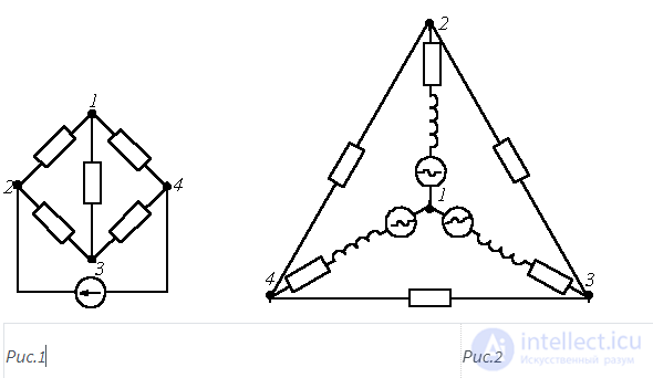
A branch is a section of a circuit carried by one and the same current.
A node is the point where three or more branches are connected.
The circuits shown differ both in form and in purpose, but each of the circuits indicated contains 6 branches and 4 nodes, connected in the same way. Thus, in terms of the geometry (topology) of the branch connections, these circuits are identical.
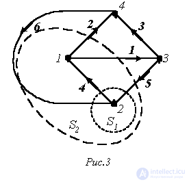
The topological (geometric) properties of an electric circuit do not depend on the type and properties of the elements that make up a branch. It is therefore convenient to represent each branch of a circuit diagram as a line segment. If each branch of the circuits in Fig. 1 and 2 is replaced by a line segment, the geometric figure shown in Fig. 3 is obtained.
The conventional representation of a circuit, in which each branch is replaced by a line segment, is called the graph of the electric circuit. It should be remembered that branches may consist of various elements, which are in turn connected in different ways.
The line segment corresponding to a circuit branch is called a branch of the graph. The boundary points of a graph branch are called nodes of the graph. The branches of a graph may be given a definite orientation, indicated by an arrow. A graph in which all branches are oriented is called a directed graph.
A subgraph of a graph is a part of the graph, i.e., it may be a single branch or a single isolated node of the graph, as well as any set of branches and nodes contained in the graph.
In circuit theory, the following subgraphs are of particular importance:
1. A path is an ordered sequence of branches in which every two adjacent branches share a common node, and any given branch and any given node occur on this path only once. For example, in the circuit of Fig. 3 the branches 2-6-5; 4-5; 3-6-4; 1 form paths between the same pair of nodes 1 and 3. Thus, a path is a set of branches traversed continuously.
2. A loop is a closed path in which one of the nodes is both the starting and the ending node of the path. For example, for the graph in Fig. 3 one can identify loops formed by the branches 2-4-6; 3-5-6; 2-3-5-4. If a connection exists between any pair of nodes of a graph, the graph is called connected.
3. A tree is a connected subgraph that contains all the nodes of the graph but no loop. Examples of trees for the graph in Fig. 3 are shown in Fig. 4.
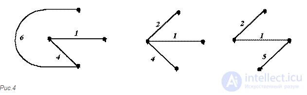
Fig.4
4. Link branches (tree complements) are the branches of the graph that complete the tree to the original graph.
If a graph contains m nodes and n branches, then the number of branches of any tree is  , and the number of link branches of the graph is
  .
.
5. A cutset of a graph is a set of branches whose removal divides the graph into two isolated subgraphs, one of which, in particular, may be a single node.
A cutset can be visually represented as the trace of some closed surface intersecting the corresponding branches. Examples of such surfaces for our graph in Fig. 3 are S1 and S2. In this case we obtain, respectively, the cutsets formed by the branches 6-4-5 and 6-2-1-5.
Associated with the concept of a tree are the concepts of principal loops and principal cutsets:
Specifying the topology of a circuit to a computer by means of a drawing is difficult, since no effective pattern-recognition programs exist. Therefore, the topology of a circuit is entered into a computer in the form of matrices, called topological matrices. Three such matrices are distinguished: the node matrix, the loop matrix, and the cutset matrix.
1. The node matrix (incidence matrix) is a table of the coefficients of the equations formed according to Kirchhoff's first law. The rows of this matrix correspond to nodes, and the columns to the branches of the circuit.
For the graph in Fig. 3 we have the number of nodes m=4 and the number of branches n=6. Then let us write the matrix AN , taking the matrix element  (i – row number; j – column number) to be 1, if branch j is connected to node i and is oriented away from it, -1, if it is oriented toward it, and 0, if branch j is not connected to nodei . Having oriented the branches of the graph in Fig. 3, we obtain
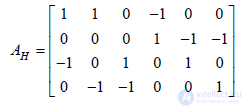
This matrix AN is written for all four nodes and is called the undetermined matrix. It should be noted that the sum of the elements of each column of matrix AN is always zero, since every column contains one element +1 and one element -1, the rest being zeros.
Usually, in calculations, one node (any one) is grounded. This brings us to the node matrix A (the reduced matrix), which can be obtained from matrix AN by deleting any one of its rows. For example, deleting row “4” gives
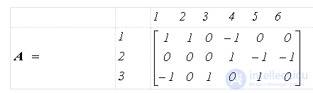
The number of rows of matrix A equals the number of independent equations for the nodes  , i.e., the number of equations written for the electric circuit by Kirchhoff's first law. So, having introduced the concept of the node matrix A, let us turn to Kirchhoff's first law.
Kirchhoff's first law
Usually Kirchhoff's first law is written for the nodes of a circuit, but, strictly speaking, it holds not only for nodes but for any closed surface, i.e., the following relation holds
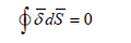 (1)
(1)
where  is the current density vector;
  is the normal to the element dS of closed surface S.
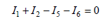
Kirchhoff's first law also holds for any cutset. In particular, for cutset S2 of the graph in Fig. 3, assuming that the numbering and directions of the currents in the branches correspond to the numbering and chosen orientation of the graph's branches, we can write
 .
.
Since, as a particular case, the branches of a cutset converge at a node, Kirchhoff's first law is valid for a node as well. For now we will apply Kirchhoff's first law to nodes, which can be written mathematically as:
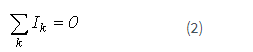
i.e., the algebraic sum of the currents of the branches connected to a node equals zero.
In calculations, the equations from Kirchhoff's first law are written for (m-1) nodes, since if equations were written for all m nodes, one of them (any one) would be linearly dependent on the others, i.e., it would give no additional information.
Let us introduce the column matrix of branch currents
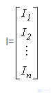
Then Kirchhoff's first law in matrix form is written as:
AI=O (3)
– where O is the zero column matrix. As we can see, the matrix A, rather than AN, is taken as the node matrix, since, as noted above, the equations from Kirchhoff's first law are written for (m-1) nodes.
As an example, let us write this for the circuit in Fig. 3
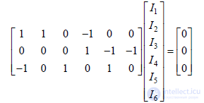
From this, for the first node we obtain

which is indeed what should hold.
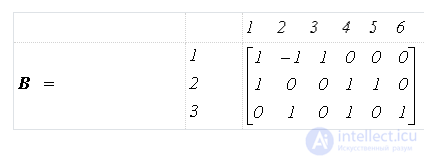
2. The loop matrix (mesh matrix) is a table of the coefficients of the equations formed according to Kirchhoff's second law. The rows of the loop matrix Bcorrespond to loops, and the columns – to the branches of the circuit.
The element bij of matrix B equals 1 if branch j belongs to loop i and its orientation coincides with the direction of traversal of the loop, -1 if it does not coincide with the direction of traversal of the loop, and 0 if branchj does not belong to loopi.
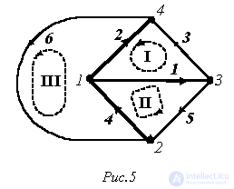
The matrix B, written for the principal loops, is called the principal-loop matrix. In this case, the direction of traversal of a loop is taken as the direction of the link branch of that loop. Selecting, in our example (see Fig. 5), the tree formed by branches 2-1-4, let us write the coefficients for matrix B.
Let us now turn to Kirchhoff's second law.
The voltage across some section of an electric circuit is understood as the difference of potentials between the endpoints of that section, i.e.

Let us sum the voltages across the branches of some loop:
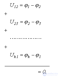
Since, in traversing a loop, the potential of each i-th point occurs twice, once with a “+” sign and once with a “-” sign, the sum as a whole equals zero.
Thus, Kirchhoff's second law is written mathematically as:
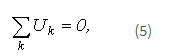
– and has the following formulation: the algebraic sum of the voltages at the terminals of the branches (elements) of a loop equals zero. In this case, when calculating circuits using Kirchhoff's laws, 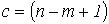 independent equations are written according to Kirchhoff's second law, i.e., equations written for loops each of which differs from the others by at least one branch. This is the significance of the topological concept of a “tree”: a tree makes it possible to form independent loops and cutsets and, consequently, to formulate independent equations from Kirchhoff's laws. Thus, taking into account the (m-1) equations formed by Kirchhoff's first law, we obtain a system of
  equations, which equals the number of branches of the circuit, and consequently the currents in them are uniquely determined.
Let us introduce the column matrix of branch voltages
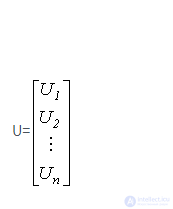
Then Kirchhoff's second law in matrix form is written as
BU = 0. (6)
As an example, for the circuit in Fig. 5 we have
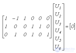
from which, for example, for the first loop we obtain
 ,
,
which is indeed what should hold.
If we introduce the column matrix of node potentials
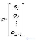
where the potential of the last node is  , then the matrix of branch voltages and node potentials are related by
|
U=AT
 |
(7)
|
where AT is the transposed node matrix.
To determine matrix B from the known matrix A=ADAC , where AD – is the submatrix corresponding to the branches of some tree, AC– is the submatrix corresponding to the link branches, the following relation can be used: B= (-ATC A-1TD1).
3. The cutset matrix – is a table of the coefficients of the equations formed according to Kirchhoff's first law for cutsets. Its rows correspond to cutsets, and its columns to the branches of the graph.
The matrix Q , formed for the principal cutsets, is called the principal-cutset matrix. The number of rows of matrix Q equals the number of independent cutsets.
The element qij of matrix Q equals 1 if the branch belongs to the i-th cutset and is oriented according to the direction of the cutset (the positive direction of a cutset is taken as the direction of the tree branch belonging to it), -1 if it is oriented opposite to the direction of the cutset, and 0 if branch j does not belong to the i-th cutset.
As an example, let us construct the matrix Q of principal cutsets for the graph in Fig. 5. With the branch orientation shown in Fig. 5, we have
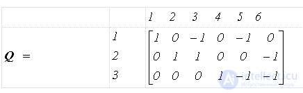
In conclusion, let us note that for the topological matrices A, B and Q, formed for one and the same graph, the following relations hold
ABT= 0; (8)
QBT= 0, (9)
which can, in particular, be used to check the correctness of the construction of these matrices. Here 0 – is a zero matrix of order  .
.
Closure or identification. It is said that a pair of vertices vi and vj in a graph G is closed (or identified) if they are replaced by a single new vertex such that all edges in graph G incident to vi and vj become incident to the new vertex.
For example, the result of closing vertices v3 and v4 in the graph of Fig.6,a is shown in Fig.6,b.
Contraction. By contraction we mean the operation of removing an edge e and identifying its end vertices. A graph G is said to be contractible to a graph H if H can be obtained from G by a sequence of contractions.
The graph shown in Fig.6,c is obtained by contracting edges e1 and e5 in graph G (Fig.6,a).
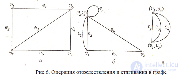
Fig.6. The operation of identification and contraction in a graph
The equations presented allow us to draw an important conclusion: knowing one of the topological matrices, the others can be reconstructed from its structure. Graph theory provides a simple, accessible, and powerful tool for building models and solving problems of ordering objects. At present there are many problems in which it is necessary to build certain complex systems by means of a specific ordering of their elements. Graph theory is of great interest to specialists in many applied disciplines. In particular, the application of this theory to the analysis of electric circuits and to the design of self-tuning fault analyzers is highly effective.
1. State the basic topological concepts for electric circuits.
2. What is the node matrix?
3. What is the loop matrix?
4. What is the cutset matrix?
5. The branch currents of some planar circuit satisfy the following complete system of independent equations:

Reconstructing the graph of the circuit, form the matrices of principal loops and cutsets, assuming that the tree branches have been assigned the first numbers.
Answer:
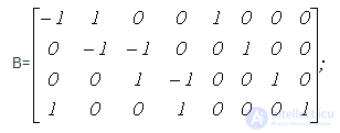
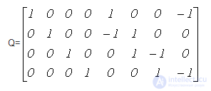
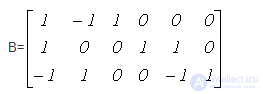
6. Construct the matrix of principal loops for the graph in Fig. 3, assuming that the tree is formed by branches 2, 1, and 5
Answer:
7. Solve problem 5 using relations (8) and (9).

Comments