
Lecture
Features of transient-process calculation in nonlinear circuits
Transient processes in nonlinear electric circuits are described by nonlinear differential equations, for which no general methods of integration exist. The superposition principle does not apply to nonlinear circuits, so methods based on it — in particular the classical method or the method using the Duhamel integral — are not applicable for calculating such circuits.
Analysis of transient regimes in electric circuits requires the use of the dynamic characteristics of nonlinear elements, which in turn depend on the dynamic processes occurring within them and, consequently, are in general not known in advance. This inherently makes the calculation of transient processes approximate to one degree or another.
A transient process in a nonlinear circuit can be characterized by a variable rate of progression over different time intervals. Therefore, the concept of a time constant is, in general, not applicable for assessing the intensity of the dynamic regime.
The lack of a unified approach to integrating nonlinear differential equations has resulted in mathematics having a large number of diverse methods for solving them, aimed at different types of equations. As applied to electrical-engineering problems, all calculation methods can, in essence, be divided into three groups:
– analytical methods, which assume either an analytical expression for the characteristics of the nonlinear elements or their piecewise-linear approximation;
– graphical methods, whose main operations are graphical constructions, often accompanied by auxiliary computational steps;
– numerical methods, based on replacing the differential equations with algebraic equations for the increments of the variables over the corresponding time intervals.
Analytical calculation methods
Analytical methods are solution methods based on the analytical integration of the differential equations describing the state of a nonlinear circuit, using analytical expressions for the characteristics of the nonlinear elements.
The main analytical methods used in solving a broad range of electrical-engineering problems are:
– the conditional linearization method;
– the analytical approximation method;
– the piecewise-linear approximation method.
Conditional linearization method
The conditional linearization method is applied in cases where, in a nonlinear equation, one of the terms on the left-hand side is small compared with the others, so that it can be suitably linearized without introducing significant error. As a result, the entire equation becomes linear with respect to one of the variables defining the characteristic  of the nonlinear element, for example
  . Using this characteristic, the time dependence
  for the second defining variable is then found by the algorithm:
 .
.
The method is notable for its simplicity; however, the solution obtained with it is fairly approximate, which is why it is mainly used for rough, order-of-magnitude calculations.
As an example of using the method, let us determine the maximum value of the current in the circuit of Fig. 1, if 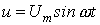 , where
  ;
;  ;
;  ;
;  . The weber-ampere characteristic of the nonlinear inductor coil is shown in Fig. 2.
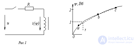
1. Let us write the state equation of the circuit after switching
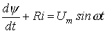 . . |
(1) |
2. Using the conditional linearization method, let us determine the second term on the left-hand side of (1) as
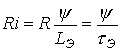 , , |
(2) |
where  ;
;  and
and  are the amplitudes of the flux linkage and current in the steady-state post-switching regime;
  .
.
3. Substituting (2) into (1), we obtain the linear differential equation
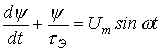 ,
,
whose solution, based on the classical method of transient-process calculation, is
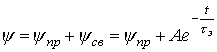 .
.
4. The forced component  is determined by the relation
 ,
,
where  .
.
To determine  and
and  , let us assume (to be verified later) that
  . Under this condition
  and
and  . From the curve
  for the obtained value
  we find
  . Then
  and
and  , i.e., the assumption made above is correct.
It should be noted that, in general, the values of  and
and  can be determined, for example, by an iterative method.
Having determined  , let us write
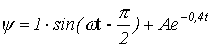 .
.
Since, by the given condition,  , then
  .
.
Thus,
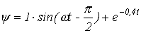 . . |
(3) |
6. Without solving the transcendental equation, let us assume that the maximum value of the flux linkage occurs approximately half a period into its variation, i.e., at  . Substituting this time into (3), we obtain:

From the curve  for
for  we find the maximum current value
  , which exceeds the amplitude of the current in the steady-state post-switching regime by a factor of
  . Recall that for a linear circuit
Notes: 1. Usually, when using the conditional linearization method to calculate the transient process upon connecting a nonlinear inductor coil to a sinusoidal-voltage source, the equivalent linear inductance  is determined from the amplitude values of the current and flux linkage in the steady-state post-switching regime, as was done in the example considered above. However, if it is necessary to estimate the maximum possible value of the current, the inductance value should be determined from the initial section of the weber-ampere characteristic, where
  is at its maximum.
2. If the resistance of the resistor in the branch with the nonlinear coil is sufficiently large, so that  , then the nonlinearity of the term
  should be neglected, setting
  . In this case the nonlinear equation (1) reduces to a linear one of the form
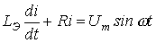 ,
,
and, correspondingly, the curve  is determined from the curves
  and
and  .
.
Analytical approximation method
The method is based on approximating the characteristic of the nonlinear element by an analytical function, which must, on the one hand, sufficiently accurately represent the original nonlinear characteristic over the range of motion of the operating point, and, on the other hand, allow for reasonably straightforward integration of the resulting differential equation (in particular, using tabulated integrals).
The method is applicable to nonlinear circuits with a single energy-storage element, described by first-order differential equations, as well as to circuits described by equations that reduce to first-order equations by a change of variables.
The value of the method lies in obtaining an expression for the quantity under study in general form, which makes it possible to carry out the required analysis of the processes when the circuit parameters are varied.
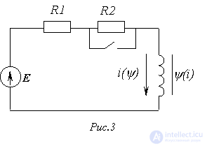
As an example of using the method, let us determine the current in the circuit of Fig. 3, assuming that the characteristic  of the nonlinear coil has the form of the typical curve in Fig. 2.
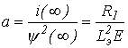
1. To solve the problem, let us choose an analytical approximation expression of the form  . Determining the parameter
  from the condition that this function corresponds to the point of the steady-state post-switching regime, we obtain
 , , |
(4) |
where  .
.
2. Substituting into the transient-process equation
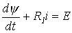
the analytical expression for the current, taking (4) into account, we obtain
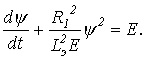 |
(5) |
Separating the variables and solving (5) with respect to time, we write
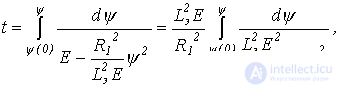 |
(6) |
where  is the initial value of the flux linkage, corresponding to the value of the current at the instant of switching
  .
.
Expression (6) corresponds to a tabulated integral; as a result we obtain
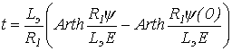 . . |
(7) |
Substituting into the last relation the expression for the flux linkage in the form
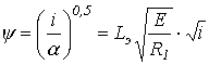 ,
,
let us rewrite (7) as

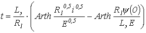 .
.
Piecewise-linear approximation method
This method is based on replacing the characteristic of the nonlinear element with straight-line segments, on the basis of which a transition is made from the nonlinear differential equation to several linear equations (one for each straight-line segment), which differ from each other only in the values of the coefficients they contain. It should be remembered that each of the linear equations is valid for the time interval during which the operating point moves along the corresponding linearized section. The time boundaries for each section are determined based on one (any) of the variables defining the characteristic of the nonlinear element reaching its boundary values for the straight-line section under consideration. In accordance with the switching laws, the values of the current in the branch with the inductor coil, or the voltage on the capacitor, at these instants of time are the initial values of the corresponding variables for the neighboring straight-line sections, on the basis of which the integration constants are determined. The value of the parameter of the linearized nonlinear element for each section of the broken line is determined by the tangent of the angle formed by the given straight-line segment with the corresponding axis of the coordinate system.
As an example, let us consider the application of this method to solve the previous problem.
1. Let us replace the operating section of the dependence  (see Fig. 2) with two straight-line segments
  and
and  . The first of them corresponds to the equation
  , the second – to
  . Here the initial point
  is determined by the current
  and the end point
  - by the current
  .
.
The inductances corresponding to these sections
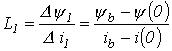 ;
;
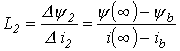 .
.
2. In accordance with the linearization indicated, the nonlinear differential state equation of the circuit
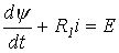
is replaced by two linear equations:
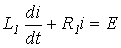 ;
;
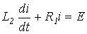 .
.
3. The solution of the first equation is
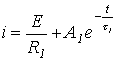
and of the second -
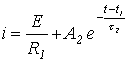 ,
,
where  ;
;  ;
;  ;
;  .
.
Let us determine the time t1, corresponding to the moment of transition from the first section to the second, from the equation
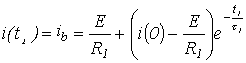 ,
,
from which
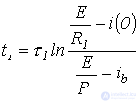 .
.
References
Review questions and problems
Answer: 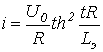 .
.
 by the expression
  , determine the current in the circuit of Fig. 1 when it is switched onto a DC voltage
  .
. , similar to
  in Fig. 2, use the piecewise-linear approximation method to determine the dependence
  .
.
Comments