
Lecture
The formal analogy between electrical and magnetic circuits noted in the previous lecture makes it possible to extend all the methods and techniques for calculating nonlinear resistive DC circuits to nonlinear magnetic circuits. For clarity, an equivalent electrical circuit of the original magnetic circuit can be constructed, and the calculation is carried out using it.
The nonlinearity of magnetic circuits is determined by the nonlinear nature of the dependence  , which is the analog of the I-V characteristic
  and is determined by the characteristic of the ferromagnetic material
  . When calculating magnetic circuits with constant flux, the basic magnetization curve is usually used. The loop-like nature of the dependence
  is taken into account when calculating permanent magnets and electrical devices based on them.
In practice, two typical problems arise when calculating magnetic circuits:
It should be noted that problems of the second type are usually more complex and laborious to solve.
In general, depending on the type of problem being solved (“direct” or “inverse”), the solution can be carried out by the following methods:
In using each of these methods, it is first necessary to indicate on the diagram the directions of the MMFs, if the directions of the currents in the windings are known, or to assume their positive directions if they need to be determined. Positive directions are then assigned to the magnetic fluxes, after which one can proceed to constructing the equivalent circuit and performing the calculations.
By configuration, magnetic circuits can be divided into unbranched and branched ones. In an unbranched magnetic circuit, the same flux exists in all its sections, i.e., the different sections of the circuit are connected in series with one another. Branched magnetic circuits contain two or more loops.
These methods are used to solve first-type problems - the ”direct” problems. Here, the input data for the calculation are the configuration and basic geometric dimensions of the magnetic circuit, the magnetization curve(s) of the ferromagnetic material, and the magnetic flux or magnetic induction in some cross section of the magnetic core. It is required to find the MMF, the winding currents, or, if the latter are known, the number of turns.
1. The ”direct” problem for an unbranched magnetic circuit
Problems of this type are solved in the following sequence:
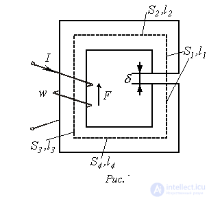
1. A mean line is drawn (see the dashed line in Fig.1), which is then divided into sections with a constant cross section of the magnetic core.
2. Based on the constancy of the magnetic flux along the entire circuit, the induction values are determined for each  -th section:
 .
.
3. From the magnetization curve, for each value of  the field strengths
  in the ferromagnetic sections are found; the field strength in the air gap is determined according to
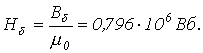
4. Using Kirchhoff's second law for the magnetic circuit, the required MMF is determined by summing the magnetic voltage drops along the loop:
 ,
,
where  is the length of the air gap.
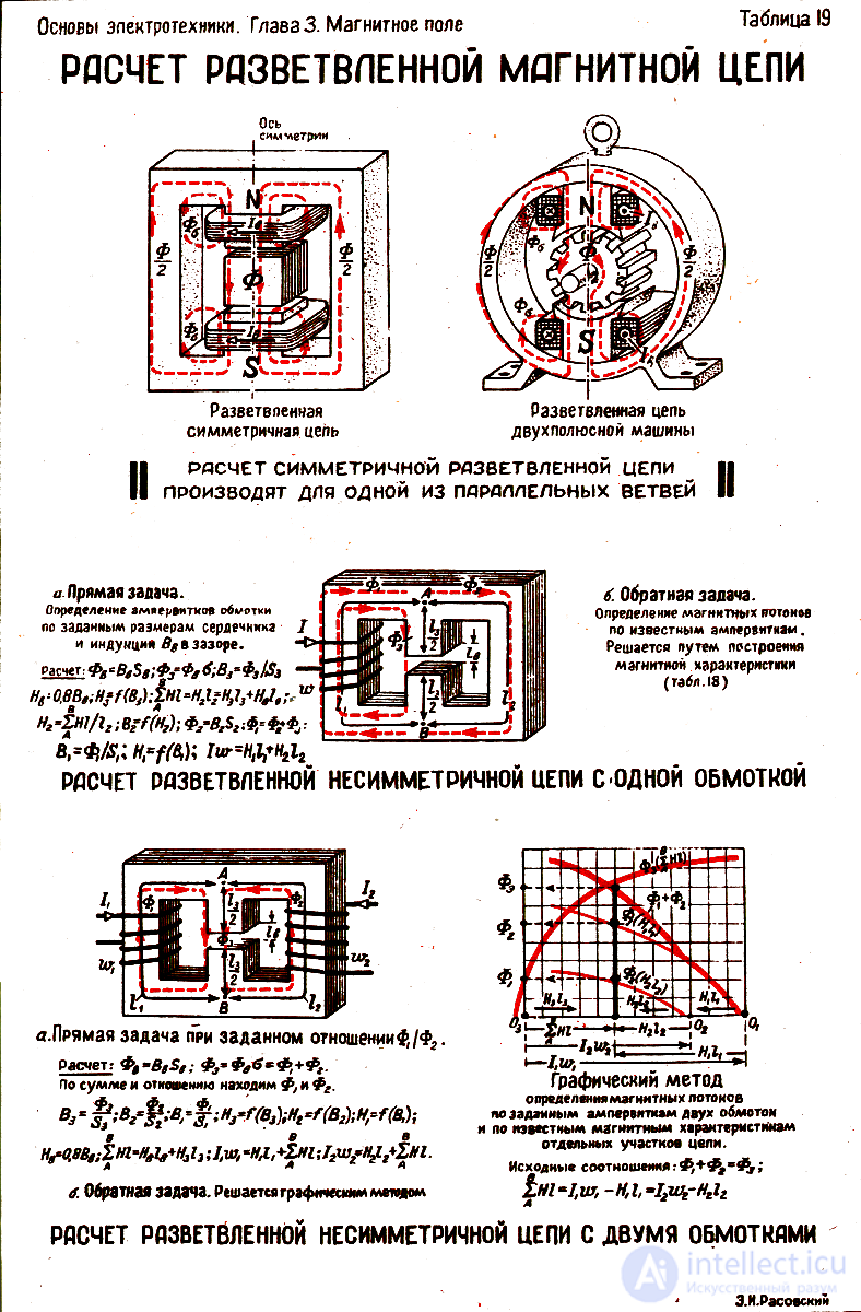
2. The "direct" problem for a branched magnetic circuit
The calculation of branched magnetic circuits is based on the combined application of Kirchhoff's first and second laws for magnetic circuits. The sequence for solving problems of this type generally corresponds to the algorithm described above for solving the "direct" problem for an unbranched circuit. In this case, to determine the magnetic fluxes in the sections of the magnetic core for which the magnetic field strength is known or can be calculated from Kirchhoff's second law, the following algorithm should be used
 |
via |  |
 |
In the remaining cases, the unknown magnetic fluxes are determined on the basis of Kirchhoff's first law for magnetic circuits.
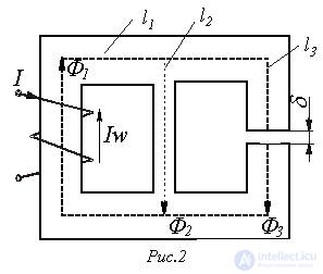
As an example of the analysis of a branched magnetic circuit, given the geometry of the magnetic circuit in Fig. 2 and the characteristic  of the ferromagnetic core, let us determine the MMF
  required to create the flux density
  in the air gap.
The algorithm for solving the problem is as follows:
1. We assign positive directions to the magnetic fluxes in the limbs of the magnetic core (see Fig. 2).
2. We determine the field strength in the air gap  and, from the relationship
  for
for  , the value
  .
.
3. Using Kirchhoff's second law for the right-hand loop, we can write

from which we find  and, from the relationship
  ,
,  .
.
4. According to Kirchhoff's first law
 .
.
Then  , and from the relationship
  we determine
  .
.
5. According to Kirchhoff's second law, the equation for the required MMF is
 .
.
Graphical calculation methods
Graphical methods are used to solve problems of the second type - "inverse" problems. In this case, the initial data for the calculation are the configuration and geometric dimensions of the magnetic circuit, the magnetization curve(s) of the ferromagnetic material, and the MMF of the windings. It is required to find the values of the fluxes (flux densities) in the individual sections of the magnetic core.
These methods are based on the graphical representation of the weber-ampere characteristics  of the linear and nonlinear sections of the magnetic circuit, followed by the solution of algebraic equations, written according to Kirchhoff's laws, by means of the corresponding graphical constructions on a plane.
1. The "inverse" problem for an unbranched magnetic circuit
Problems of this type are solved in the following sequence:
1. Values of the flux are assumed and, for them, the MMF  is determined, as when solving the "direct" problem. In this case, one should try to select two sufficiently close flux values so as to obtain
  , one slightly less and one slightly greater than the given MMF value.
2. Using the data obtained, part of the characteristic  magnetic circuit (near the given MMF value), and from it the flux corresponding to the given MMF value is determined.
When calculating unbranched magnetic circuits containing air gaps, it is convenient to use the intersection method, in which the required solution is determined by the point of intersection of the nonlinear weber-ampere characteristic of the nonlinear part of the circuit and the linear characteristic of the linear section, constructed on the basis of the equation

where  is the magnetic reluctance of the air gap.
2. The "inverse" problem for a branched magnetic circuit
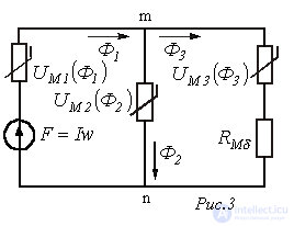
Replacing the magnetic circuit with an equivalent electrical circuit (see Fig. 3, which shows the equivalent circuit of the magnetic circuit of Fig. 2) makes it possible to solve problems of this type using all the graphical methods and techniques applied in the analysis of similar nonlinear DC electrical circuits.
In this case, when calculating magnetic circuits containing two nodes (this configuration is found in a large number of magnetic cores used in practice), the two-node method is widely used. The idea behind this method is similar to that considered for nonlinear resistive DC circuits and consists of the following:
1. The relationships  for the fluxes in all
  branches of the magnetic circuit are calculated as a function of the total magnetic voltage
  between nodes
  and
and  .
.
2. The point at which Kirchhoff's first law  is graphically satisfied is determined. The fluxes corresponding to this point are the solution to the problem.
These methods, the essence of which was discussed in the analysis of nonlinear resistive DC circuits, are approximate numerical techniques for solving the nonlinear algebraic equations describing the state of a magnetic circuit. As noted above, they are readily amenable to computer algorithmization and are now widely used in the study of complex magnetic circuits on digital computers. For the analysis of relatively simple circuits containing a small number of nodes and nonlinear elements in the equivalent electrical circuit (usually up to two or three), it is possible to implement the methods "by hand".
As an example, let us give the algorithm for calculating the magnetic circuit in Fig. 1, in which, given the geometry of the magnetic core, the characteristic  of the core material, and the MMF value F, it is necessary to find the flux Φ.
In accordance with the step-by-step calculation, for this circuit we can write
 , , |
(1) |
where  .
.
We assume a value of  , calculate
  for the
  sections of the magnetic core, find
  from the magnetization curve
  , compute
  , and use (1) to determine
  for the next approximation, and so on, until the equality
  is satisfied to within the given tolerance.
Static and differential inductance of a coil
with a ferromagnetic core
Let us consider a coil with a ferromagnetic core, shown in Fig. 4.
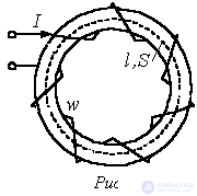
In accordance with the definition of flux linkage
 , , |
(2) |
and, based on the total current law  , from which
 . . |
(3) |
From relations (2) and (3) it follows that the function  qualitatively has the same form as
  . Thus, the relationships for the relative magnetic permeability
  and the inductance
  are also similar, i.e., the curves
  and
and  shown in the previous lecture in Fig. 2 are qualitatively analogous to the curves
  and
and  .
.
Static inductance of a coil with a ferromagnetic core
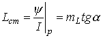 ;
;
differential inductance
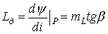 .
.
If the magnetic permeance of the core in Fig. 4 is denoted by  , then
  and
and  , from which
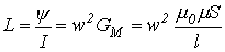 |
(4) |
Using relation (4), let us show the effect of the air gap on the inductance of the coil.
Let the coil in Fig. 4 have an air gap  . Then the total magnetic reluctance of the loop is
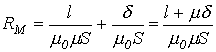 ,
,
from which
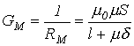 .
.
For  , consequently
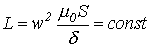 .
.
Thus, the air gap linearizes the coil with a ferromagnetic core. A gap for which the inequality  holds is called a large gap.
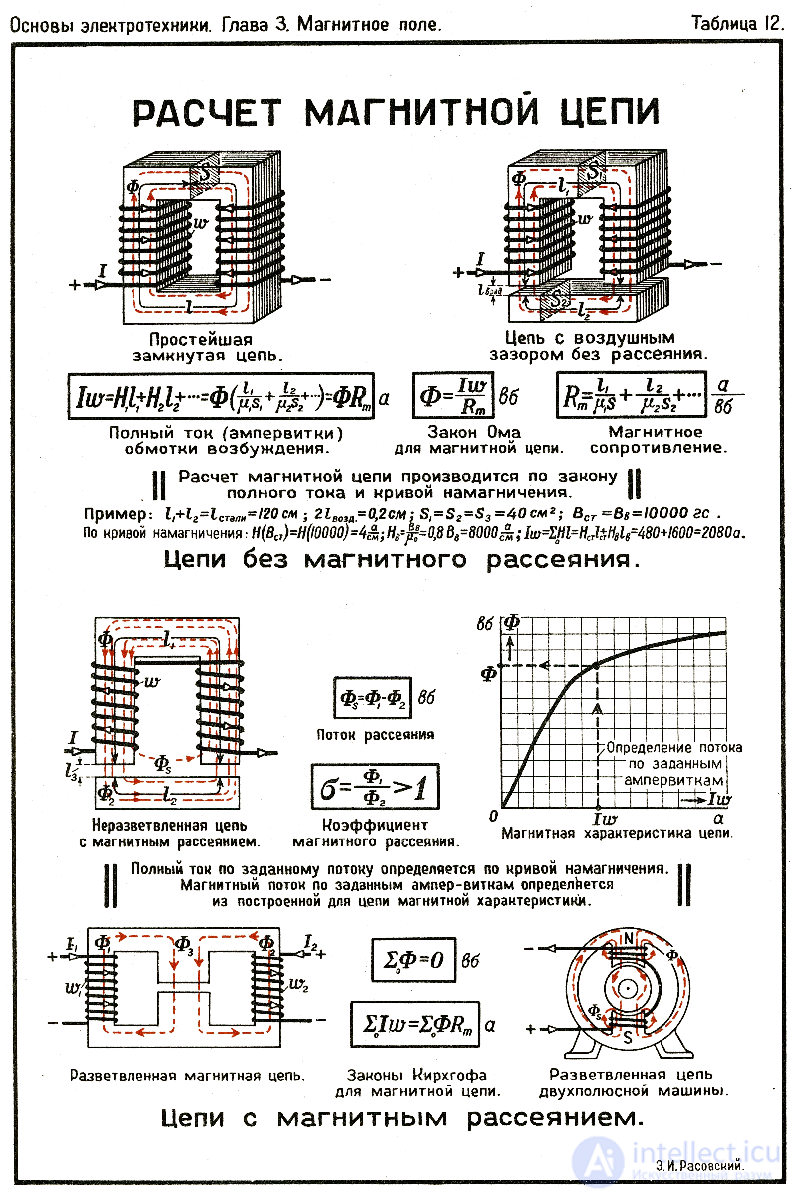
 and
and  are given. Devise an algorithm for calculating the length of the air gap
  .
. .
. and differential
  inductances.
Comments