
Lecture
Distributed-parameter circuits - are electrical circuits in which the voltages and currents at different points of even an unbranched circuit differ from one another, i.e. they are functions of two independent variables: time t and the spatial coordinate x.
Electromagnetic waves propagate at a finite speed. This
gives the processes occurring in electrical circuits a wave-like character, i.e.
the currents and voltages in an electrical circuit turn out to depend not only on
time t, but also on the coordinate x of the circuit's cross-section, i.e. U(x,t); i(x,t).
• If λ>L, then it is a lumped-parameter circuit.
• If λ at the same time it has the properties of R, L, C elements, i.e. the parameters of the elements are, as it were, distributed over the entire section of the circuit.
Examples of distributed-parameter circuits:
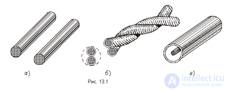
In previous lectures we considered electrical circuits whose geometric dimensions, as well as those of the elements comprising them, played no role, i.e. the electric and magnetic fields were localized within the capacitor and the inductor, respectively, and the power loss was localized in the resistor. In practice, however, one often has to deal with circuits (power-transmission lines, information-transmission lines, windings of electrical machines and apparatus, etc.) in which the electromagnetic field and the losses are distributed uniformly or nonuniformly along the entire circuit. As a result, the voltages and currents at different points of even an unbranched circuit differ from one another, i.e. they are functions of two independent variables: time t and the spatial coordinate x. Such circuits are called distributed-parameter circuits. The meaning of this name lies in the fact that for circuits of this class, every infinitesimally small element of their length is characterized by a resistance and an inductance, while between the conductors there is, respectively, a capacitance and a conductance.
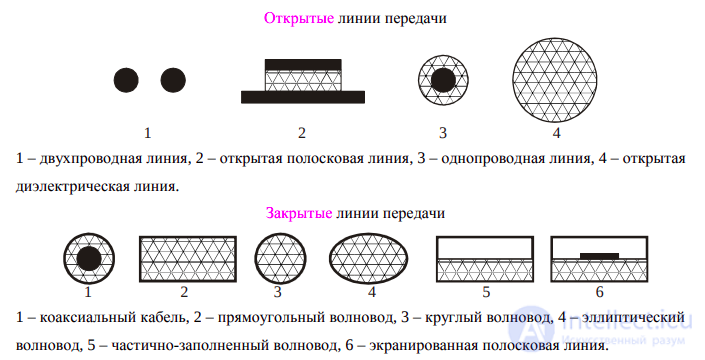
To assess which type a circuit belongs to – lumped or distributed parameters – its length l should be compared with the wavelength of the electromagnetic wave  . If
. If  , then the line should be regarded as a distributed-parameter circuit. For example, for
  , i.e. at
  , and
, and  . For
. For  , i.e. already at
  the line should be treated as a distributed-parameter circuit.
To study the processes in a distributed-parameter circuit (also called a long line), let us introduce the additional condition that its parameters – inductance, resistance, capacitance, and conductance – are uniformly distributed along the line. Such a line is called homogeneous. A line with a nonuniform distribution of parameters can often be divided into homogeneous sections.
Long lines are characterized by primary parameters, that is, parameters referred to a unit length of the line. The primary parameters include: 1. The resistance per unit length of the line  .
.
2. The inductance per unit length of the line  .
.
3. The capacitance per unit length of the line  .
.
4. The conductance per unit length of the line 
By the primary parameters of the line we mean the resistance  , the inductance
  , the conductance
  and the capacitance
  , referred to a unit of its length. To obtain the equations of a homogeneous line, let us divide it into individual sections of infinitesimal length
  with the structure shown in Fig. 1.
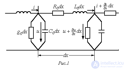
Let the voltage and current at the beginning of such an elementary two-port be u and i, and at the end, respectively,  and
and  .
.
The difference between the voltages at the beginning and end of the section is determined by the voltage drop across the resistive and inductive elements, while the change in current over the section equals the sum of the leakage and displacement currents through the conductance and capacitance. Thus, by Kirchhoff's laws
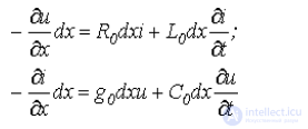
or, after dividing by 
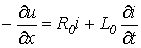 ; ; |
(1) |
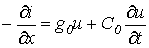 . . |
(2) |
We will consider the theory of distributed-parameter circuits in steady-state regimes for the case of sinusoidal current. The relations obtained can then be extended, at  , to DC circuits, and, using a Fourier-series expansion, to lines carrying periodic nonsinusoidal current.
Introducing complex quantities and replacing  with
with  , on the basis of (1) and (2) we obtain
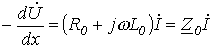 ; ; |
(3) |
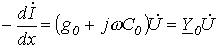 , , |
(4) |
where  and
and  are, respectively, the complex impedance and admittance per unit length of the line.
Differentiating (3) with respect to x and substituting the expression  from (4), we write
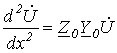 .
.
The characteristic equation
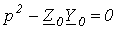 ,
,
whence
 .
.
Thus,
 , , |
(5) |
where  is the propagation constant;
  is the attenuation coefficient;
  is the phase coefficient.
For the current, according to equation (3), we can write
 , , |
(6) |
where 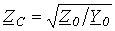 is the characteristic (wave) impedance.
The characteristic impedance  and the propagation constant
  are called the secondary parameters of the line, which characterize its properties as a device for transmitting energy or information.
Defining  and
and  , on the basis of (5) we write
 . . |
(7) |
A similar equation, according to (6), can be written for the current.
The terms on the right-hand side of relation (7) can be interpreted as traveling waves: the first moves and decays in the direction of increasing x, the second in the direction of decreasing x. Indeed, at a fixed instant of time each term is a (owing to energy losses) decaying harmonic function of the coordinate x, while at a fixed point it is a sinusoidal function of time.
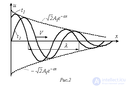
The wave moving from the beginning of the line in the direction of increasing x is called the forward (incident) wave, while the one moving from the end of the line in the direction of decreasing x is called the backward (reflected) wave.
Fig. 2 shows the decaying sinusoid of the forward wave for the time instants  and
and 
 . The motion of the wave is characterized by the phase velocity. This is the speed of propagation along the line of an unchanged phase state, i.e., the speed at which one must move along the line in order to observe the same phase of the wave:
 . . |
(8) |
Differentiating (8) with respect to time, we obtain
 . . |
(9) |
The wavelength  is the distance between its two nearest points that differ in phase by
  rad. In accordance with this definition
 ,
,
whence

and taking (9) into account
 .
.
In accordance with the concepts introduced for the forward and backward waves, the voltage distribution along the line at any instant of time can be interpreted as the result of the superposition of two waves – forward and backward – traveling along the line with the same phase velocity but in opposite directions:
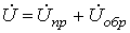 , , |
(10) |
where, in accordance with (5),  and .
and .
Representing the voltage as the sum of the forward and backward waves according to (10) means that the positive directions of the voltage for both waves are chosen the same way: from the upper conductor to the lower one.
Similarly, for the current, based on (6), we can write
 , , |
(11) |
where 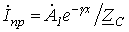 and
and  .
.
The positive directions of the forward and backward current waves according to (11) are different: the positive direction of the forward wave coincides with the positive direction of the current  (from the beginning to the end of the line), while the positive direction of the backward wave is opposite to it.
On the basis of (10) and (11), Ohm's law holds for the forward and backward voltage and current waves
 |
 |
Let us consider the theoretically important case of an infinitely long homogeneous line.
In the case of an infinitely long line, in expressions (5) and (6) for the voltage and current, the terms containing  must be absent, since letting
  deprives these terms of physical meaning. Consequently, in the case under consideration
  . Thus, in the solution of the equations of an infinitely long line there are no backward waves of current and voltage. In accordance with the above
 |
 |
(12) |
On the basis of relations (12), an important conclusion can be drawn: for an infinitely long line, at any point on it, including the input, the ratio of the complex voltage and current is a constant quantity equal to the characteristic impedance:
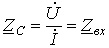 .
.
Thus, if such a line is mentally cut at any point and, instead of the discarded infinitely long portion, an impedance numerically equal to the characteristic impedance is connected, the operating mode of the remaining finite-length section will not change. From this, two conclusions can be drawn:
The equations of the infinitely long line extend to a finite-length line loaded with an impedance equal to the characteristic impedance. In this case as well, only forward waves of voltage and current exist.
For a line loaded with the characteristic impedance, the input impedance is also equal to the characteristic impedance.
The operating mode of a long line loaded with an impedance equal to the characteristic impedance is called matched, and the line itself is called a line with a matched load.
Note that this mode is practically important for information transmission, since it is characterized by the absence of reflected (backward) waves, which cause interference.
A matched load completely absorbs the power of the wave that has reached the end of the line. This power is called the natural power. Since at any cross-section of a matched line the impedance equals the characteristic impedance, the phase-shift angle  between voltage and current is unchanged. Thus, if the power received by the line from the generator equals
  , then the power at the end of a line of length
  in this case is
 ,
,
whence the efficiency of the line
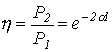
and the attenuation
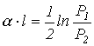 .
.
As noted when discussing two-port networks, the unit of attenuation is the neper, which corresponds to a power attenuation of  times, and a voltage or current attenuation of
  times.
The most typical applications of long lines are:
1) Communication means (means of transmitting signals from a signal source to a load).
2) Delay line.
If the line is loaded with an impedance equal to the characteristic impedance, and at the instant t = 0 the signal source produces a rectangular pulse, then, because of the finite propagation speed of the signal 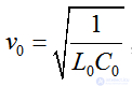 , where L0, C0 are the per-unit-length parameters, the signal will appear at the load with a delay, where td = L/v0. Since the line is loaded with the characteristic impedance Zw, no signal distortion occurs. If Zw = ZL, the signal is observed with distortion of its shape.
3) Impedance transformer:
a) Quarter-wave impedance transformer.
Let us consider a section of long line whose length is a quarter of the wavelength: L = λ/4, loaded with a resistive impedance RL. The input impedance of such a section is given by the relation
Zin = ρ2/ RL.
It follows that, by varying the ratio ρ/RL, the input impedance of the line can be changed over a wide range. If it is necessary to transform the impedance RL into R1L, then the impedance RL must be connected through a quarter-wave section with a characteristic impedance ρ = (RL R1L)1/2.
b) Metallic insulator.
The expression for the input impedance – of a quarter-wave line section – shows that at RL = 0 its input impedance is infinite. This makes it possible to use it as an insulator.
c) Resonant circuit.
In microwave radio engineering, instead of resonant circuits made up of L, C-elements, two-terminal networks in the form of short-circuited sections are used. The input impedance of a short-circuited line section is determined as
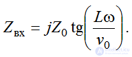 .
.
If l = λ/2, then Zin = ∞, i.e. a quarter-wave section of a long line short-circuited at the end has properties analogous to a parallel resonant circuit.
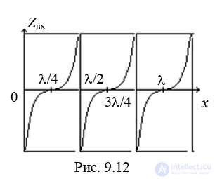
Let us determine the frequencies at which the line section behaves as a parallel resonant circuit, i.e., has a maximum of the impedance magnitude

From this 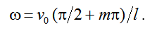 . At these frequencies this section will behave as a parallel resonant circuit (Fig. 9.12).
4) Short rectangular pulse shaper.
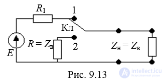
If a DC voltage source E (Fig. 9.13) is connected to a matched long line, the same voltage is established along its entire length – the line is charged (the switch is in position 1).
If the switch is thrown to position 2, a rectangular voltage pulse is formed across the impedance R = Zw, whose duration equals twice the delay time of the line.
 .
. ,
,  and
and  for a cable for which
  ,
, 
 , if the frequency is
  .
.



 .
. ;
; 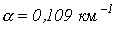 ;
;  .
.

Comments