
Lecture
In the analysis of electric circuits, in problems studying the relationship between variables (currents, voltages, powers, etc.) of two branches of a circuit, two-port network theory is widely used. A two-port network is a part of a circuit of arbitrary configuration having two pairs of terminals (hence its name), usually called the input and output terminals.
Examples of two-port networks are a transformer, an amplifier, a potentiometer, a transmission line and other electrical devices in which two pairs of terminals can be distinguished.
In general, two-port networks can be divided into active ones, whose structure includes energy sources, and passive ones, whose branches contain no energy sources.
Below, the elements of the theory of passive two-port networks will be considered.
To write the equations of a two-port network, let us isolate, in an arbitrary circuit, a branch with a single energy source and any other branch with some resistance  (see Fig. 1,a).
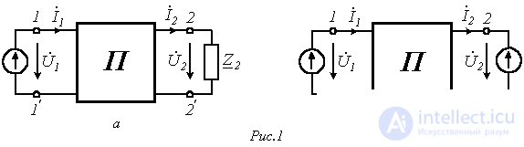
In accordance with the compensation principle, let us replace the original resistance  by a source with voltage
  (see Fig. 1,b). Then, on the basis of the superposition method, for the circuit in Fig. 1,b we can write
 ; ; |
(1) |
 . . |
(2) |
Solving the equations (1) and (2) obtained for the voltage and current at the primary terminals, we get
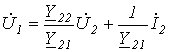 ;
;

or
 ; ; |
(3) |
 , , |
(4) |
where  ;
;  ;
;  ;
;  - the coefficients of the two-port network.
Considering that, in accordance with the reciprocity principle,  , it can be seen that the coefficients of the two-port network are related to each other by
 . . |
(5) |
Equations (3) and (4) are the basic equations of a two-port network; they are also called the equations of the two-port network in A-form (see Table 1). In general, there are six forms of writing the equations of a passive two-port network. Indeed, a two-port network is characterized by two voltages  and
and  and two currents
  and
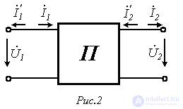
and  . Any two of these quantities can be expressed through the remaining two. Since the number of combinations of four taken two at a time equals six, there are also six possible forms of writing the equations of a passive two-port network, which are given in Table 1. The positive directions of the currents for the different forms of the equations are shown in Fig. 2. Note that the choice of one form of the equations or another is determined by the area and type of problem being solved.
Table 1. Forms of writing the equations of a passive two-port network
|
Form |
Equations |
Relation to the coefficients of the basic equations |
|
A-form |
|
|
|
Y-form |
|
|
|
Z-form |
|
|
|
H-form |
|
|
|
G-form |
|
|
|
B-form |
|
|
If, when the source and the receiver of energy are interchanged, their currents do not change, such a two-port network is called symmetric. As can be seen from comparing the A- and B-forms in Table 1, this holds when  .
.
Two-port networks that do not satisfy this condition are called asymmetric.
For the practical use of the two-port network equations in circuit analysis, it is necessary to know the values of its coefficients. The coefficients of a two-port network can be determined either experimentally or by calculation. In this case, in accordance with relation (5), determining any three coefficients makes it possible to determine the fourth as well.
One of the most convenient experimental methods for determining the coefficients of a two-port network is based on open-circuit and short-circuit tests with the network fed from the secondary terminals, and an open-circuit test with the network fed from the primary terminals. In this case, at  , on the basis of equations (3) and (4)
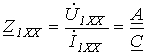 . . |
(6) |
At 
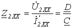 |
(7) |
and at 
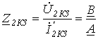 . . |
(8) |
Solving equations (6)-(8) for the coefficients of the two-port network gives:

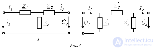
When the coefficients of a two-port network are determined by calculation, the connection scheme and the values of the resistances of the two-port network must be known. As noted earlier, a passive two-port network is characterized by three independent constant coefficients. Consequently, a passive two-port network can be represented as a three-element equivalent T-shaped (Fig. 3,a) or Π-shaped (Fig. 3,b) equivalent circuit.
To determine the coefficients of the two-port network for the circuit in Fig. 3,a, using Kirchhoff's first and second laws, let us express  and
and  in terms of
  and
and  :
:
 ; ; |
(9) |
 . . |
(10) |
Comparing the expressions (9) and (10) obtained with relations (3) and (4) gives:

This problem can also be solved in another way. At  (open circuit on the secondary side), in accordance with (3) and (4)
 and
and  ;
;
but from the circuit in Fig. 3,a
 , and
, and  ;
;
from which it follows that:  and
and  .
.
At  (short circuit at the secondary terminals)
 and
and  .
.
From the circuit in Fig. 3,a
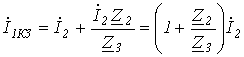 ;
;
 .
.
Consequently, 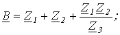
 .
.
Thus, the same results are obtained as in the first case.
The coefficients of the two-port network for the circuit in Fig. 3,b can be determined in a similar way, or on the basis of those obtained for the circuit in Fig. 3,a, using the previously discussed “star-delta” transformation formulas.
From the above, it can be concluded that, knowing the coefficients of the two-port network, one can always find the parameters of its T- and Π-shaped equivalent circuits.
In practice, it is often necessary to go from one form of writing the two-port network equations to another. To solve this problem, i.e. to determine the coefficients of one form of the equations through the coefficients of another, one should express any two identical quantities in these formulas through the other two, and compare them, taking into account the positive directions of the currents for each of these forms. Thus, when going from the A- to the Z-form, on the basis of (4) we have
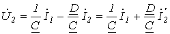 . . |
(11) |
Substituting relation (11) into (3) gives
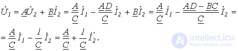 . . |
(12) |
Comparing expressions (11) and (12) with the two-port network equations in Z-form (see Table 1), we obtain
 .
.
When analyzing the operation of a two-port network on a load  , it is convenient to use the concept of input resistance on the primary side
  and the transfer coefficient
  . Considering that
  and
and 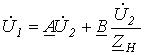 , for these parameters we can write:
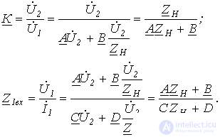
Knowing  ,
,  and
and  , one can determine the remaining variables at the input and output of the two-port network:
  ;
;  ;
;  .
.
Characteristic impedance and propagation
coefficient of a symmetric two-port network
In telecommunications, the operating mode of a symmetric two-port network is widely used, in which its input resistance equals the load resistance, i.e.
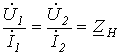 .
.
This resistance is denoted as  and is called the characteristic impedance of the symmetric two-port network, and the operating mode of the two-port network for which
 ,
,
is called the matched-load mode.
In the indicated mode, for a symmetric two-port network  , on the basis of (3) and (4) we can write
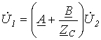 ; ; |
(13) |
 . . |
(14) |
Dividing relation (13) by (14), we obtain the equation
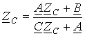 ,
,
the solution of which is
 . . |
(15) |
Taking (15) into account, equations (13) and (14) take the form
 ;
;
 .
.
Thus,
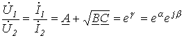 ,
,
where  - the propagation coefficient;
  - the attenuation coefficient (measured in nepers);
  - the phase coefficient (measured in radians).
One neper corresponds to an attenuation in voltage or current by a factor of e=2.718…, and, since for the case under consideration  , an attenuation in power by a factor of e2.
Let us write the equation of a symmetric two-port network using the propagation coefficient.
By definition
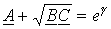 . . |
(16) |
Then
 . . |
(17) |
Solving (17) and (18) for  and
and  , we obtain
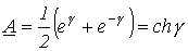 and
and 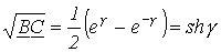 .
.
Considering that
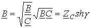
and
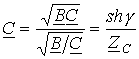 ,
,
we obtain the equations of the two-port network written in terms of hyperbolic functions:
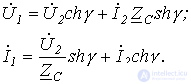
References
Review questions and problems
Answer:  ;
;  ;
;  ;
;  .
.
Determine the parameters of the T-shaped equivalent circuit.
Answer:  ;
;  ;
;  .
.
Determine at what load resistance the input resistance of the two-port network will equal the load resistance.
Answer:  .
.
 ;
;  ;
; 
 ;
;  .
.





















Comments