
Lecture
Circuits are called nonlinear if they contain at least one nonlinear element.
Elements are called nonlinear if their parameters depend on the magnitude and (or) direction of the variables associated with these elements (voltage, current, magnetic flux, charge, temperature, luminous flux, etc.). Nonlinear elements are described by nonlinear characteristics, which have no strict analytical expression, are determined experimentally, and are given in tabular or graphical form.
Nonlinear elements can be divided into two-terminal and multi-terminal ones. The latter contain three (various semiconductor and electron triodes) or more (magnetic amplifiers, multi-winding transformers, tetrodes, pentodes, etc.) terminals, by means of which they are connected to the electric circuit. A characteristic feature of multi-terminal elements is that, in general, their properties are determined by a family of characteristics representing the dependence of the output characteristics on the input variables and vice versa: input characteristics are plotted for a series of fixed values of one of the output parameters, and output characteristics for a series of fixed values of one of the input parameters.
According to another classification criterion, nonlinear elements can be divided into inertial and inertialess. Inertial elements are those whose characteristics depend on the rate of change of the variables. For such elements, the static characteristics, which determine the relationship between the rms (root-mean-square) values of the variables, differ from the dynamic characteristics, which establish the relationship between the instantaneous values of the variables. Inertialess elements are those whose characteristics do not depend on the rate of change of the variables. For such elements, the static and dynamic characteristics coincide.
The concepts of inertial and inertialess elements are relative: an element can be regarded as inertialess within a permissible (upper-bounded) frequency range, beyond which it passes into the category of inertial elements.
Depending on the type of characteristic, nonlinear elements are distinguished as having symmetric and asymmetric characteristics. A characteristic is called symmetric if it does not depend on the direction of the quantities that define it, i.e. it is symmetric with respect to the origin of the coordinate system:  . For an asymmetric characteristic this condition is not satisfied, i.e.
  . The presence of a symmetric characteristic in a nonlinear element makes it possible, in a number of cases, to simplify the analysis of the circuit by carrying it out within a single quadrant.
By the type of characteristic, all nonlinear elements can also be divided into elements with single-valued and multi-valued characteristics. A characteristic  is called single-valued if each value of x corresponds to a single value of y and vice versa. In the case of a multi-valued characteristic, some values of x may correspond to two or more values of y, or vice versa. For nonlinear resistors, the ambiguity of the characteristic is usually associated with the presence of a falling section, for which
  , while for nonlinear inductive and capacitive elements it is associated with hysteresis.
Finally, all nonlinear elements can be divided into controlled and uncontrolled ones. Unlike uncontrolled elements, controlled nonlinear elements (usually three- and multi-terminal ones) contain control channels; by varying the voltage, current, luminous flux, etc. in these channels, their main characteristics – the voltage-current, weber-ampere, or coulomb-voltage characteristic – are changed.
Nonlinear DC electric circuits
The nonlinear properties of such circuits are due to the presence of nonlinear resistors in them.
Because nonlinear resistors lack direct proportionality between voltage and current, they cannot be characterized by a single parameter (a single value of  ). In the general case, the relationship between these quantities depends not only on their instantaneous values but also on their derivatives and integrals with respect to time.
Parameters of nonlinear resistors
Depending on the operating conditions of the nonlinear resistor and the nature of the problem, static, differential, and dynamic resistance are distinguished.
If the nonlinear element is inertialess, it is characterized by the first two of the parameters listed.
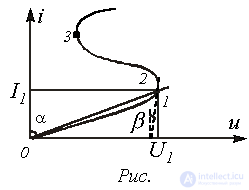
The static resistance equals the ratio of the voltage across the resistive element to the current flowing through it. In particular, for point 1 of the V-A characteristic (VAC) in fig. 1
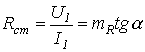 .
.
The differential resistance is understood as the ratio of an infinitesimal increment of voltage to the corresponding increment of current
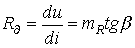 .
.
It should be noted that for an uncontrolled nonlinear resistor  is always positive, whereas
  can also take negative values (section 2-3 of the VAC in fig. 1).
In the case of an inertial nonlinear resistor, the concept of dynamic resistance is introduced
 ,
,
determined from the dynamic VAC. Depending on the rate of change of the variable, for example the current, not only the magnitude but also the sign of  can change.
Methods for calculating nonlinear DC electric circuits
The electrical state of nonlinear circuits is described on the basis of Kirchhoff's laws, which are general in nature. It should, however, be remembered that the superposition principle is not applicable to nonlinear circuits. For this reason, the calculation methods developed for linear circuits on the basis of Kirchhoff's laws and the superposition principle do not, in general, extend to nonlinear circuits.
There are no general methods for calculating nonlinear circuits. The known techniques and approaches have varying capabilities and areas of application. In general, when analyzing a nonlinear circuit, the system of nonlinear equations describing it can be solved by the following methods:
Graphical calculation methods
When using these methods, the problem is solved by graphical constructions on a plane. In doing so, the characteristics of all branches of the circuit should be written as functions of one common argument. Owing to this, the system of equations is reduced to a single nonlinear equation with a single unknown. For calculation purposes, circuits with series, parallel, and mixed connections are formally distinguished.
a) Circuits with series-connected resistive elements.
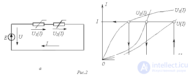
For a series connection of nonlinear resistors, the current flowing through the series-connected elements is taken as the common argument. The calculation is carried out in the following sequence. From the given VACs  of the individual resistors, a resulting relationship
  is plotted in the system of Cartesian coordinates
  . Then, on the voltage axis, a point is marked corresponding, on the chosen scale, to the given value of the voltage at the input of the circuit, from which a perpendicular is erected until it intersects the relationship
  . From the point where the perpendicular intersects the curve
  , an orthogonal is dropped onto the current axis – the resulting point corresponds to the sought current in the circuit, and from the value of this current found, using the relationships
  , the voltages
  across the individual resistive elements are determined.
Application of this procedure is illustrated by the graphical constructions in fig. 2,b, corresponding to the circuit in fig. 2,a.
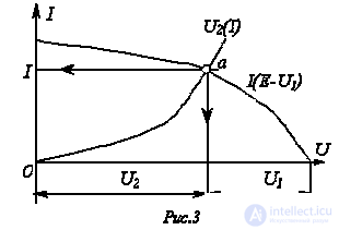
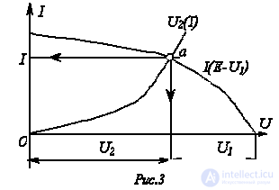
The graphical solution for a series nonlinear circuit with two resistive elements can also be carried out by another method – the intersection method. In this case one of the nonlinear resistors, for example the one with VAC  in fig.2,a, is regarded as the internal resistance of a source with EMF E, and the other as the load. Then, on the basis of the relation
  , point a (see fig. 3), the intersection of the curves
  and
and  , determines the operating mode of the circuit. The curve
  is constructed by subtracting the abscissas of the VAC
  from the EMF E for various values of the current.
The use of this method is most rational for a series connection of a linear and a nonlinear resistor. In this case the linear resistor is taken as the internal resistance of the source, and the linear VAC of the latter is constructed from two points.
b) Circuits with parallel-connected resistive elements.
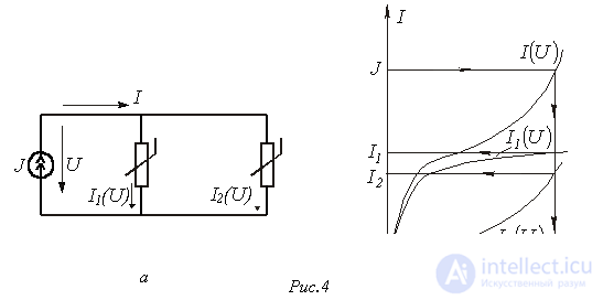
For a parallel connection of nonlinear resistors, the voltage applied to the parallel-connected elements is taken as the common argument. The calculation is carried out in the following sequence. From the given VACs  of the individual resistors, a resulting relationship
  is plotted in the system of Cartesian coordinates
  . Then, on the current axis, a point is marked corresponding, on the chosen scale, to the given value of the source current at the input of the circuit (if there is a voltage source at the input of the circuit, the problem is solved directly by erecting a perpendicular from the point corresponding to the given source voltage until it intersects the VAC
  ), from which a perpendicular is erected until it intersects the relationship
  . From the point where the perpendicular intersects the curve
  , an orthogonal is dropped onto the voltage axis – the resulting point corresponds to the voltage across the nonlinear resistors, and from the value found, using the relationships
  , the currents
  in the branches with the individual resistive elements are determined.
The use of this procedure is illustrated by the graphical constructions in fig. 4,b, corresponding to the circuit in fig. 4,a.
c) Circuits with series-parallel (mixed) connection of resistive elements.
1. The calculation of such circuits is carried out in the following sequence:
The original circuit is reduced to a circuit with series-connected resistors, for which purpose the resulting VAC of the parallel-connected elements is constructed, as shown in item b).
2. The resulting circuit with series-connected resistive elements is calculated (see item a), on the basis of which the currents in the original parallel branches are then determined.
Two-node method
For circuits containing two nodes, or reducible to such, the two-node method can be applied. In a fully graphical implementation of the method, it consists of the following:
Graphs of the dependences  of the currents in all i-th branches are plotted as a function of the common quantity – the voltage
  between nodes m and n; to do this, each of the original curves
  is shifted along the voltage axis, parallel to itself, so that its origin lies at the point corresponding to the EMF
  in the i-th branch, and is then mirrored about the perpendicular erected at that point.
The point at which Kirchhoff's first law  is graphically satisfied is determined. The currents corresponding to this point are the solution of the problem.
The two-node method can also be implemented in another variant, requiring fewer graphical constructions than the one described above.
As an example, consider the circuit in Fig. 5. For it, we express the voltages across the resistive elements as a function of  :
:
 ; ; |
(1) |
 ; ; |
(2) |
 . . |
(3) |
Next, we assign a value to the current flowing through one of the resistors, for example in the second branch  , and calculate
  , then, using
  together with (1) and (3), we find
  and
and  , and from the dependences
  and
and  - the corresponding currents
  and
and  , etc. The calculation results are collected in Table 1, in whose last column we determine the sum of the currents
 .
.
Table 1. Table of calculation results using the two-node method
|
|
|
|
|
|
|
|
|
According to Kirchhoff's first law, the algebraic sum of the currents must equal zero, so the value  obtained in the last column of Table 1 indicates what value of
  should be assigned at the next step.
In the  axes we plot the curve
  and, from the point where it crosses the voltage axis, determine the voltage
  between points m and n. For the value of
  found, we use (1)…(3) to calculate the voltages across the resistors, after which, from the given dependences
  , we determine the currents in the branches of the circuit.
References
Review Questions and Problems
Answer:  .
.
Answer:  .
.
Answer:  .
.
 and
and  , where voltage is in volts and current is in amperes;
  . Using the graphical method, determine the voltages across the resistors.
 and
and  , where current is in amperes and voltage is in volts;
  . Using the graphical method, determine the currents
  and
and  .
.
 , where current is in amperes and voltage is in volts; the third resistor is linear with
  . Determine the currents in the branches using the two-node method if
  .
.






Comments