
Lecture
Graphical methods are methods based on graphical constructions in a plane. Compared with the analytical methods discussed above, they have the following main advantages:
The main drawback of graphical methods is that the solution is obtained for specific values of the circuit parameters.
The main graphical methods used in solving electrical-engineering problems are:
1. Graphical integration method
The graphical integration method is based on the graphical evaluation of a definite integral and consists in successively finding the areas under the curve of the corresponding integrand function. It is applied to the analysis of electric circuits whose transient processes are described by first-order differential equations with separable variables.
2. Isocline method
This method is one of the most widely used graphical methods of approximate integration. It is used directly to solve first-order equations of the form  and generally includes the following steps, in general:
in the plane  , using the isocline equations
  (an isocline is a line of equal slope, along which the function
  has a constant value, i.e., the locus of points for which
  ), isoclines are constructed for various values of the slope coefficient
  ;
;
along each isocline, short strokes are drawn with a slope determined by the corresponding value of  ;
;
starting from the point  corresponding to the initial condition, an integral curve is constructed so that it crosses each isocline parallel to the strokes drawn on it; the resulting curve is the graph of the sought dependence
3. Phase-plane method
The method makes it possible to carry out a qualitative study of dynamic processes in nonlinear circuits described by first- and second-order differential equations. In doing so, without directly integrating the nonlinear differential equations, this method makes it possible to obtain an understanding of the process as a whole. In general, studies carried out by the phase-plane method make it possible to reveal the dependence of the character of the transient process on the initial conditions, to judge the stability or instability of the circuit's operation, to establish the possibility of self-oscillations arising in the circuit with an assessment of their frequency and shape, and so on.
A more detailed treatment of graphical methods can be found in [1,2,3].
Numerical methods for calculating transient processes
Numerical methods for analyzing dynamic processes in nonlinear electric circuits are based on various numerical techniques for the approximate integration of nonlinear differential equations. They are based on a general principle: the original differential equation is replaced by an algebraic equation for the increments of the dependent (studied) variable over the corresponding intervals of change of the independent variable (time).
The main advantage of numerical methods is their universality, i.e., their fundamental suitability for analyzing any circuit. This is especially important in the case of nonlinear circuits, for which no general analytical calculation methods exist.
As applied to the analysis of dynamic processes in nonlinear circuits, the most widely used are:
The state-variable method, as was shown in the analysis of transient processes in linear circuits, is based on formulating and integrating differential equations written in normal form. The complete system of equations in matrix form has the form
 = =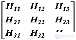 . . |
(1) |
Here  and
and  are the matrices of the state variables and their first time derivatives, respectively; w(z) is the matrix of nonlinear resistive elements; z is the matrix of arguments of the nonlinear resistive elements; v is the matrix of input excitations (source EMFs and currents); y is the matrix of the sought quantities.
When formulating the state equations for relatively simple circuits, they can be written directly from Kirchhoff's laws. In the general case, however, either a procedure based on constructing a connection table according to a special algorithm is used for this purpose — as was shown when discussing the state-variable method as applied to the calculation of linear circuits — or a procedure based on the superposition principle.
Procedure for formulating the state equations based on the superposition principle
This procedure for formulating the state equations follows from splitting the original circuit into two subcircuits:
An example of such a representation of the original circuit is shown in Fig. 1,a, where the passive multi-terminal network P corresponds to the second subcircuit.
The next stage of the procedure under consideration consists in replacing, on the basis of the compensation theorem, all capacitors, as well as nonlinear resistive elements with a characteristic of the type u(i), by voltage sources, and all inductor coils and nonlinear resistive elements with a characteristic of the type i(u) by current sources (Fig. 1,b). As a result, the original circuit is transformed into a resistive one, in which, besides the given (independent) sources, controlled sources are also acting.
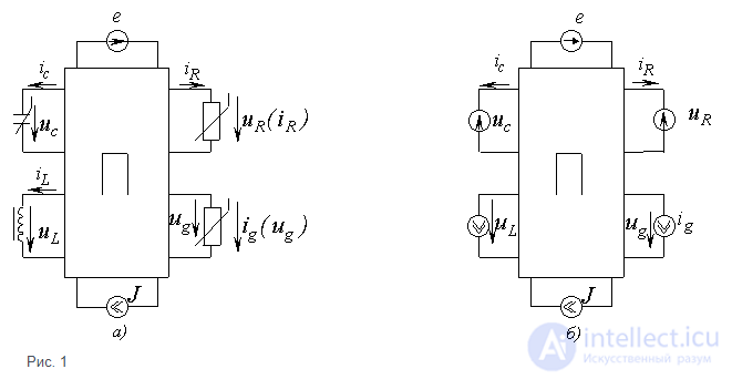
At the third stage, using the superposition method, expressions are determined for the input currents and voltages of the passive multi-terminal network P in terms of the voltages and currents of all the sources connected to it.
As an example, let us formulate the state equations for the circuit in Fig. 2,a and determine the expressions  and
and  .
.
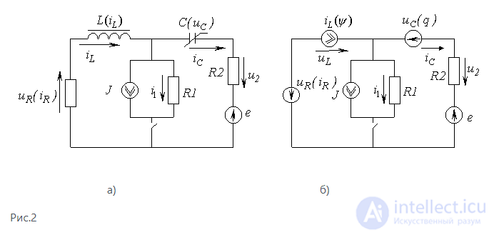
1. In accordance with the procedure described, let us replace the original circuit with the equivalent circuit in Fig. 2,b. Based on the superposition method, this circuit corresponds to five circuits shown in Fig. 3. Using them, for the current  =dq/dt in the branch with the capacitor and the voltage
  at the terminals of the inductor coil, let us write
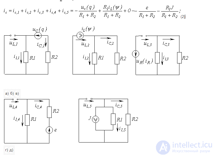
Fig. 3
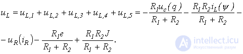 |
(3) |
2. The expression for the required voltage  is determined according to Ohm's law:
 |
( 4) |
Using the superposition method with the equivalent circuits of Fig. 3, for the second unknown variable – the current  – we write

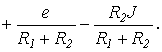 ( 5)
( 5)
3. Combining (2)  (5) and taking
  into account, we obtain the matrix equation of the form (1):
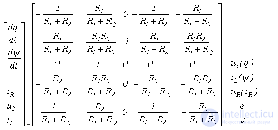
The vector of initial values 
 =
= 
 .
.
Comparing the state-equation formulation methods considered above, it can be noted that the method based on the superposition principle does not include the fairly complex step of eliminating resistive-branch variables from the state equations, which is part of the method based on the connection table. At the same time, using the superposition method for complex circuits can also turn out to be a very laborious task.
Discrete-model method
The method is based on using discrete models of the inductive and capacitive elements and makes it possible to reduce the numerical analysis of dynamic processes in nonlinear circuits to a sequential calculation of nonlinear resistive circuits at each step.
Discrete models follow from implicit algorithms, in particular from the backward Euler formula. These models, obtained on the basis of the implicit Euler algorithm, together with the expressions for the parameters of the elements they contain, are given in Table 1.
Table 1. Discrete models of the inductive and capacitive elements
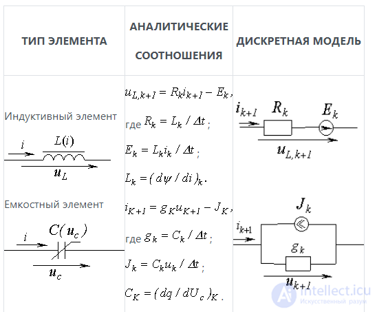
Note: if the capacitive and inductive elements are linear and  then
then  and
and  .
.
The discrete-model method lends itself well to computer algorithmization and is used to calculate complex nonlinear circuits on a computer. For sufficiently simple circuits it can be implemented ’’by hand’’.
The sequence of calculating a nonlinear circuit by the discrete-model method is illustrated by the example problem solution below.
In the circuit of Fig. 3 from the previous problem, the source EMF E = 1 V;  1 Ohm;
  4 Ohm. The weber-ampere characteristic of the nonlinear inductor is approximated by the expression
  where the current is in amperes and the flux linkage is in webers.
Calculate the current i in the circuit after the switch closes
Solution
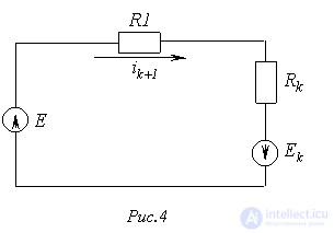
1. Let us draw the discrete equivalent circuit for the calculation (see Fig. 4).
For this circuit we have
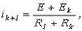 |
(6) |
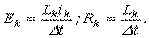
where, in accordance with Table 1
The value of the differential inductance of the nonlinear coil at the k-th step
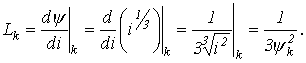 |
(7) |
2. Let us choose the integration step  Based on the commutation law

Then 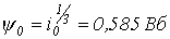 and, in accordance with (7),
  .
.
Parameters of the equivalent-circuit elements: 
 whence, on the basis of (6)
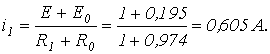
At the next step  then
then  and the parameters of the equivalent-circuit elements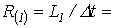

 whence
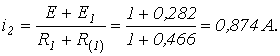
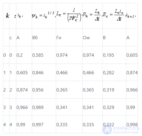
The results of the step-by-step calculation according to the algorithm above are presented in Table 2.
Table 2. Calculation results

Comments