
Lecture
If a complex electrical circuit contains a single branch with a nonlinear resistor, the current in that branch can be determined on the basis of the active two-terminal network theorem (the equivalent-generator method). The idea of the solution is as follows. The branch containing the nonlinear resistor is separated from the original circuit, and the remaining, now linear, network is represented as an active two-terminal network (ATN). According to the ATN theorem, the linear ATN, as seen from terminals 1-2 of the separated branch (see Fig. 1,a), can be represented by an equivalent generator (see Fig. 1,b) with an EMF equal to the voltage  at terminals 1-2 with the branch containing the nonlinear resistor open-circuited, and with an internal resistance equal to the input resistance of the linear two-terminal network.
The resulting circuit is calculated, for example, by the graphical method, as a circuit with series-connected elements.
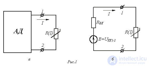
If it is also necessary to find the currents in the linear part of the original circuit, then after calculating the nonlinear circuit of Fig. 1,b, in accordance with the compensation theorem, the nonlinear resistor is replaced by an EMF or current source, after which the resulting linear circuit is analyzed by any known method.
Analytical calculation methods
It is convenient to study the general properties of nonlinear circuits on the basis of mathematical analysis relying on an analytical expression for the characteristics of nonlinear elements, i.e., their approximation. The choice of analytical method is influenced by the conditions of the problem at hand, as well as by the nature of the possible movement of the operating point along the characteristic of the nonlinear element: over the entire characteristic or within a relatively small region of it.
The analytical methods include:
The analytical approximation method is based on replacing the characteristic (or a portion of it) of the nonlinear element with a general analytical expression. The following types of analytical approximation are used:
The coefficients (a,b,c,…) are chosen so as to give the best fit of the analytical expression to the working portion of the nonlinear characteristic. In doing so
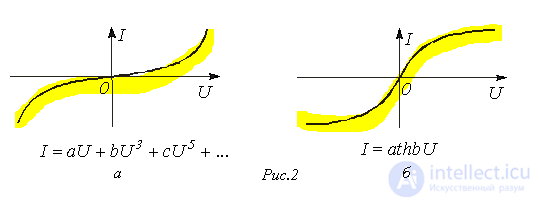
the most characteristic points through which the analytical curve must pass are selected. The number of points equals the number of coefficients in the analytical expression, which makes it possible to determine the latter uniquely.
It must be remembered that when several roots of the nonlinear equation are obtained, they must be checked for whether they satisfy the problem. Suppose, for example, that in a circuit consisting of a linear resistor R and a nonlinear resistor connected in series, the I-V characteristic of the latter can be approximated by the expression  . Determine the current in the circuit if the EMF source E ensures that the circuit operates in the first quadrant.
According to Kirchhoff's second law, the following equation holds for this circuit

or
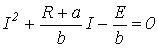 .
.
The roots of the equation
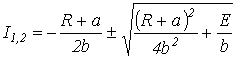 .
.
The solution to the problem is  , since the second solution
  does not satisfy the conditions on physical grounds.
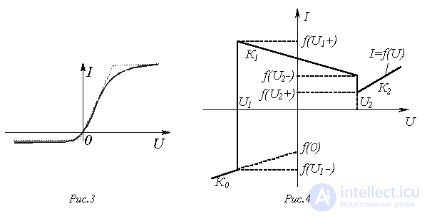
The piecewise-linear approximation method is based on representing the characteristic of a nonlinear element by straight-line segments (see Fig. 3), as a result of which the nonlinear circuit can be described by linear equations with coefficients that are constant within each segment.
When a circuit contains two or more nonlinear resistors, implementing this method is difficult, since in the general case it is not known in advance which segments of the piecewise curves the operating points lie on.
Piecewise-linear approximation can be implemented using the method of sectional piecewise-linear functions, which makes it possible to describe the broken-line curve by a single general analytical expression. For example, for the curve shown in Fig. 4 and defined by the coefficients  and
and  characterizing the slope of its individual straight-line segments, and the parameters

 , characterizing the coordinates of the points where the function values change abruptly, this expression will have the form
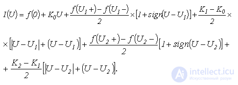
Here the first two terms on the right-hand side define the first sloped segment of the approximated curve; the first three terms define the first sloped segment together with the first jump; the first four terms define the first and second sloped segments together with the first jump, and so on.
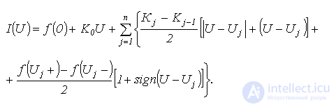
In the general case, the approximating expression obtained by the method of sectional piecewise-linear functions has the form
The linearization method is applicable for analyzing nonlinear circuits under small deviations of the operating point P (see Fig. 5) from its initial state.
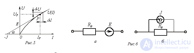
In the vicinity of the operating point  (see Fig. 5)
 ,
,
where  (Ohm's law for small increments);
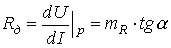 -differential resistance.
The idea of the method is to replace the nonlinear resistor with a linear one whose resistance equals the differential resistance at the given (or assumed) operating point, together with either a series-connected EMF source or a parallel-connected current source. Thus, the linearized I-V characteristic (see the straight line in Fig. 5) corresponds to a series (Fig. 6,a) or parallel (Fig. 6,b) equivalent circuit of the nonlinear resistor.
If the initial operating condition is known and it is only necessary to calculate the increments of currents and (or) voltages caused by a change in the source voltage or current, it is expedient to use equivalent circuits for the increments, obtained on the basis of Kirchhoff's laws for small increments:
 ;
; .
.When constructing the circuit for the increments:
1) all EMFs and source currents are replaced by their increments;
2) nonlinear resistors are replaced by linear ones with resistances equal to the differential resistances at the operating points.
It must be remembered that the total value of any current or voltage in the circuit equals the algebraic sum of the initial value of the variable and its increment calculated by the linearization method.
If the initial operating condition of the nonlinear resistor is unknown, an operating point on its I-V characteristic should be assumed and, after performing the corresponding linearization, the calculation should be carried out; at its conclusion it is necessary to check whether the results correspond to the chosen point. If they do not match, the linearized segment is refined and the calculation is repeated, and so on until the required convergence is achieved
Iterative calculation methods
The solution of the nonlinear equation (system of nonlinear equations) describing the state of the electrical circuit can be obtained by approximate numerical methods. The solution is found as follows: based on an initial, sufficiently rough, estimate, the starting value of the root (roots) is determined, after which it is refined according to the chosen algorithm until it falls within the specified error tolerance.
The methods most widely used in electrical engineering for the numerical calculation of nonlinear resistive circuits are the simple iteration method and the Newton-Raphson method, the basic information about which is given in Table 1.
Table 1. Iterative calculation methods
Calculation sequence
1.The original nonlinear equation of the electrical circuit  , where
  is the unknown variable, is represented in the form
  .
.
2. The calculation is carried out using the algorithm  where
where  - iteration step.
Geometric illustration of the algorithm
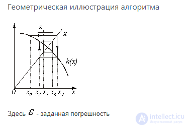
Here  - specified error tolerance
Iteration convergence condition
On the interval between the approximate and exact values of the root, the inequality must hold 
Note
1.The initial approximation  is usually found from the equation
  by neglecting the nonlinear terms in it.
2. The method can be extended to a system of nonlinear equations of order n. For example, when solving a 2nd-order system
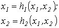
the iteration formulas have the form  ;
;  .
.
Calculation sequence
1. Based on the original nonlinear equation of the electrical circuit  , where
  is the unknown variable, the iteration formula
 is written, where
  - iteration step.
2.Using the formula obtained, the iterative calculation is carried out
Geometric illustration of the algorithm
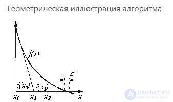
Here - specified error tolerance
Iteration convergence condition
On the interval between the approximate and exact values of the root, the inequalities must hold 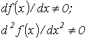
Note
Notes 1, 2, and 3 for the simple iteration method also apply to the Newton-Raphson method. In this case, when solving a 2nd-order system 
the iteration formulas have the form
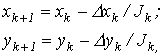
where
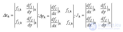
Answer: P=2 W.
Answer:  .
.
Answer:  ;
;  .
.
Answer:  .
.
 , where
  . The linear resistances of opposite arms of the bridge are pairwise equal:
  ;
;  . Determine the power dissipated by the nonlinear resistor if the circuit is fed from a source with EMF
  .
. and a nonlinear resistor connected in series, if the I-V curve of the latter
  passes through the points with coordinates (15 V; 1.425 A) and (5 V; 0.325 A) and is approximated by an expression of the form
  . The EMF at the input of the circuit is
  .
. ;
;  ;
;  . Determine the voltage
  across the nonlinear resistor and the current
  through it using the Newton-Raphson method.
 ,
,  . The I-V characteristic of the nonlinear resistor is approximated by two straight-line segments, the first of which passes through the points with coordinates (0 V; 0 A) and (9 V; 2 A), and the second – through the points with coordinates (9 V; 2 A) and (12 V; 6 A). Determine the current in the circuit.

Comments