
Lecture
A set of radius vectors representing sinusoidally varying EMFs, voltages, currents, etc. is called a phasor diagram. Phasor diagrams clearly illustrate the course of solving a problem. With an accurate construction of the vectors, the amplitudes and phases of the required quantities can be determined directly from the diagram. An approximate (qualitative) construction of the diagrams during an analytical solution serves as a reliable check on the correctness of the solution process and makes it easy to determine the quadrant in which the vectors being found are located.
When constructing phasor diagrams for circuits with series-connected elements, the current vector should be taken as the base (reference) vector (see Lecture No. 8), and the voltage vectors across the individual elements are plotted relative to it at the corresponding angles. For circuits with parallel-connected elements, the voltage vector should be taken as the base (reference) vector (see Lecture No. 8), with the current vectors in the parallel branches oriented relative to it.
To clearly determine the magnitude and phase of the voltage between different points of an electric circuit, it is convenient to use topographic diagrams. They are points on the complex plane, connected according to the circuit diagram, representing the potentials of those points. In a topographic diagram, which is in essence a phasor diagram, the order in which the voltage vectors are arranged strictly corresponds to the order in which the elements are arranged in the circuit, and the voltage-drop vector across each successive element is attached to the end of the voltage vector of each preceding element.
As an example, let us construct the current phasor diagram, as well as the topographic diagram of potentials, for the circuit whose calculation was given in Lecture No. 5 (see Fig. 1).
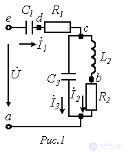
Circuit parameters: 



For these parameters and the given input voltage of the circuit  , the current values found (see Lecture No. 5) are:
  ;
; 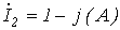 ;
;  .
.
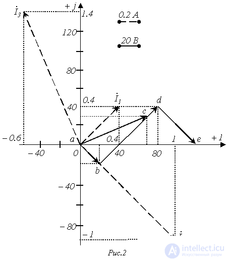
When constructing the phasor diagram, let us choose scales for the currents and voltages (see Fig. 2). A phasor diagram can be constructed from a complex quantity written in exponential form, i.e. from its magnitude and phase values. In practice, however, it is more convenient to carry out the construction using the algebraic form, since in this case the real and imaginary components of the complex quantity are plotted directly on the corresponding axes of the complex plane, determining the position of the point on it.
The construction of the current phasor diagram is carried out directly on the basis of the known values of their complex representations. To construct the topographic diagram, we first calculate the complex potentials (another way of constructing the topographic diagram involves calculating the complex voltages across the circuit elements, followed by summing the voltage vectors along the loop directly on the complex plane).
When constructing the topographic diagram, the loop can be traversed in the direction of the current or against it. The second option is used more often.
In this case, taking into account that in electrical engineering it is accepted that current flows from higher to lower potential, the potential of the point being sought equals the potential of the preceding point plus the voltage drop across the element between these points. If an EMF source is encountered along the path of traversal, the potential of the point being sought will equal the potential of the preceding point plus the value of this EMF, if the direction of traversal coincides with the direction of the EMF, and minus the value of the EMF if it does not. This follows from the fact that the voltage across an EMF source has a direction opposite to the EMF.
Denoting on the circuit of Fig. 1 the points between the circuit elements as e and a, and taking the potential of point a as zero (  ), let us determine the potentials of these points:

or 

Thus, as a result of the calculations performed, we obtain that  . But the potential difference between points e and a equals the voltage U applied to the circuit, and it equals 120 V. Thus, Kirchhoff's second law is satisfied, and consequently the calculations have been performed correctly. In accordance with the results obtained, the topographic diagram in Fig. 2 is constructed. Attention should be paid to the orientation of the vectors making up the topographic diagram relative to the current vectors: for resistive elements the corresponding vectors are parallel, while for the inductive and capacitive elements they are orthogonal.
In conclusion, note that the voltage vectors are oriented relative to the points of the topographic diagram opposite to the positive directions of the voltages relative to the corresponding points of the electric circuit. In this connection, it is permissible not to indicate the directions of the voltage vectors on the topographic diagram.
Potential diagram
The potential diagram is used in the analysis of DC circuits. It is a graph of the potential distribution along a section of a circuit or a loop, where the resistances of the resistive elements encountered along the path of traversal of the branch or loop are plotted on the abscissa axis, and the potentials of the corresponding points are plotted on the ordinate axis. Thus, each point of the section or loop under consideration corresponds to a point on the potential diagram.
Let us consider the construction of a potential diagram using the circuit in Fig. 3 as an example.
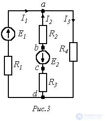
With the circuit parameters  ;
;  ;
;  ;
;  ;
;  and
and  , the currents in the circuit branches are:
  ;
;  ;
;  .
.
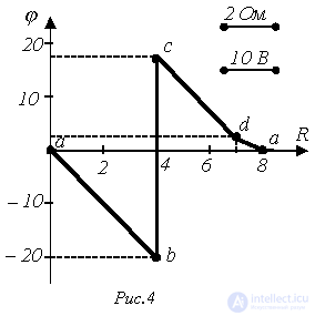
Let us construct the potential diagram for loop abcda.
To choose the scale for the abscissa axis, let us sum the resistances of the resistors along the loop under consideration: 
 after which we determine the potentials of the loop points relative to the potential of an arbitrarily chosen point a, whose potential is taken as zero:
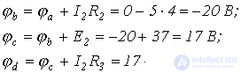
Thus, the coordinates of the points of the potential diagram are: a(0;0);b(4;-20); c(4;17); d(7;2). Taking the chosen scales into account, the potential diagram for the selected loop is constructed in Fig. 4.
Transformation of linear electric circuits
To simplify the calculation and increase the clarity of the analysis of complex electric circuits, it is in many cases rational to subject them to a preliminary transformation. Obviously, the transformation should lead to a simplification of the original circuit by reducing the number of its branches and (or) nodes. Such a transformation is called expedient. In this case, whatever the method of transformation, the condition of unchanged currents in the branches of the parts of the circuit not affected by these transformations must hold. It follows from this that if the transformed sections of the circuit contain no energy sources, the powers in the original and equivalent circuits are the same. If the transformed sections include energy sources, then in the general case the powers in the original and transformed circuits will differ.
Let us consider the most important cases of transformation of electric circuits.
1. Transformation of series-connected elements
Consider the section of the circuit in Fig. 5,a. When calculating the part of the circuit external to this section, this branch can be reduced to the form in Fig. 5,b, where
 |
(1) |
or
 . . |
(2) |

Here, when calculating the equivalent EMF  , the k-th EMF is taken with a “+” sign if its direction coincides with the direction of the equivalent EMF, and with a “-” sign if it does not.
2. Transformation of parallel-connected branches
Suppose we have the circuit in Fig. 6,a.
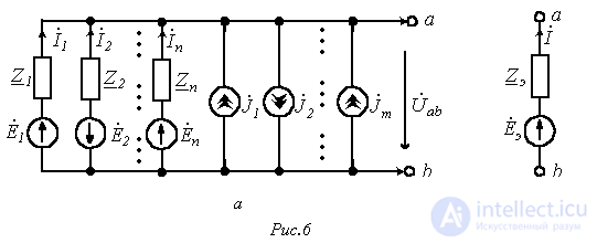
According to Ohm's law for a section of a circuit with an EMF source
 ,
,
where  .
.
Then
 ,
,where
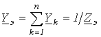 ; ; |
(3) |
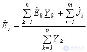 , , |
(4) |
moreover, the EMF  and current
  are written with a “+” sign in (4) if they are directed toward the same node as the EMF
  ; otherwise they are written with a “-” sign.
3. Mutual "delta-star" transformations
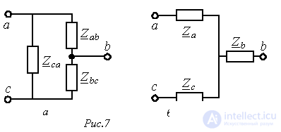
In a number of cases, circuits may be encountered in which the connections cannot be classified as either series or parallel (see Fig. 7). In such cases the transformations are more complex in nature: transformation of a delta into a star and vice versa.
To transform a delta into a star means to replace three resistances connected in a delta between some three nodes with three other resistances connected in a star between the same points. In this case, the currents in the parts of the circuit not affected by these transformations must remain unchanged.
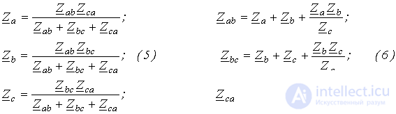
Without derivation, let us write the formulas for the equivalent transformations
|
Delta |
Star |
References
Review questions and problems
Answer:  .
.
Answer:  ;
;  ;
;  .
.
Answer:  ;
;  ;
;  .
.
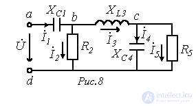
 and the parameters of all its elements are known in the circuit of Fig. 8, qualitatively construct the current phasor diagram and the potential topographic diagram for it.
 .
. ,
,  and
and  .
. star
star
Comments