
Lecture
Suppose the signal that needs to be transmitted along the line without distortion is periodic, i.e., it can be expanded in a Fourier series. The signal will be distorted if the attenuation and phase velocity are different for its harmonic components, i.e., if the latter are functions of frequency. Thus, for there to be no distortion – which is very important, for example, in information-transmission lines – it is necessary that all harmonics propagate with the same velocity and the same attenuation, since only in that case, when superimposed, do they form a signal at the end of the line similar to the input signal.
Ideal in this case is the so-called lossless line, for which the resistance  and the conductance
  are equal to zero.
Indeed, in this case
 ,
,
i.e., regardless of frequency the attenuation coefficient  and the phase velocity
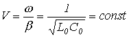 .
.
However, distortion can also be absent in a line with losses. The condition for distortionless signal transmission follows from a joint consideration of the expressions for the propagation constant
 |
(1) |
and the phase velocity
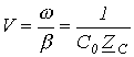 . . |
(2) |
From (1) and (2) it follows that, in order to obtain  and
and  , which ensures the absence of distortion, it is necessary that
  , i.e., that the characteristic impedance be independent of frequency.
 . . |
(3) |
As the analysis of (3) shows, at
 |
(4) |
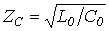 is a real constant.
A line whose parameters satisfy condition (4) is called a distortionless line.
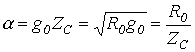
The phase velocity for such a line
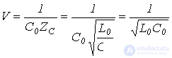
and the attenuation
 .
.
It should be noted that for real lines (both overhead and cable lines)  . Therefore, to impart the properties of a distortionless line to real lines, their inductance is artificially increased by inserting special loading coils at equal intervals, and, in the case of cable lines, also by wrapping the conductors with a ferromagnetic tape.
Equations of a finite-length line
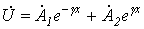
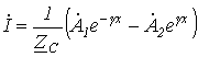
The constants  and
and  in the formulas obtained in the previous lecture
 ; ; |
(5) |
 |
(6) |
are determined from the boundary conditions.
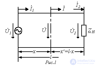
Suppose that for a line of length l (see Fig. 1) the voltage  and current
  at the beginning of the line, i.e. at
  , are given.
Then from (5) and (6) we obtain
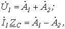
whence
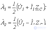
Substituting the expressions found for  and
and  into (5) and (6), we obtain
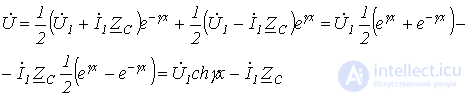 |
(7) |
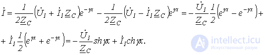 |
(8) |
Equations (7) and (8) make it possible to determine the current and voltage at any point of the line from their known values at the beginning of the line. In practical problems, the voltage  and current
  at the end of the line are usually given instead. To express the voltage and current in the line in terms of these quantities, let us rewrite equations (5) and (6) in the form
 ; ; |
(9) |
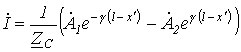 . . |
(10) |
Denoting  and
and  , from equations (9) and (10), at
  we obtain
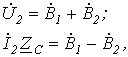
whence
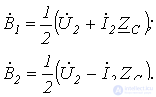
After substituting the expressions found for  and
and  into (9) and (10), we obtain equations that make it possible to determine the current and voltage from their values at the end of the line
 ; ; |
(11) |
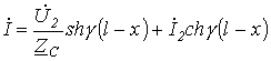 . . |
(12) |
Equations of a long line as a two-port network
In accordance with (11) and (12), the voltages and currents at the beginning and end of the line are related by
 ;
;
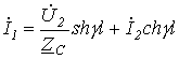 .
.
These equations correspond to the equations of a symmetric two-port network, whose coefficients are 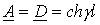 ;
;  and
and 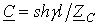 ; and the condition
  holds.
This means that the elements of two-port network theory can be applied to long lines, and, consequently, like any symmetric two-port network, a long line can be represented by a symmetric T- or Π-shaped equivalent circuit.
Determining the parameters of a long line from open-circuit
and short-circuit tests
As with two-port networks, the parameters of a long line can be determined from open-circuit (OC) and short-circuit (SC) tests.
At OC,  and
and  , whence the input impedance
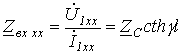 . . |
(13) |
At SC, 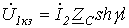 and
and  . Consequently,
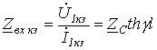 . . |
(14) |
On the basis of (13) and (14)
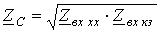 |
(15) |
and
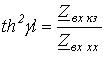 ,
,
whence
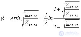 . . |
(16) |
Expressions (15) and (16), based on experimental data, make it possible to determine the secondary parameters  and
and  of the line, from which its primary parameters
  and
and  can then be calculated.
Lossless line
A lossless line is a line whose primary parameters  and
and  are equal to zero. In this case, as was shown earlier,
  and
and 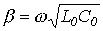 . Thus,
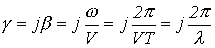 ,
,
whence  .
.
Let us expand the hyperbolic functions of the complex argument  :
:

Then, for a lossless line, i.e. at  , the following relations hold:
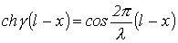 and
and 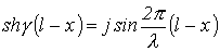 .
.
Thus, the equations of a long line in hyperbolic functions of a complex argument, for a lossless line, transform into equations written using circular trigonometric functions of a real argument:
 ; ; |
(17) |
 . . |
(18) |
Strictly speaking, a lossless line (a distributed-parameter circuit without losses) is an idealized case. However, when  and
and  hold, which is the case, for example, for high-frequency circuits, the line can be regarded as lossless and, consequently, described by equations (17) and (18).
Standing waves in long lines
As shown above, the solution of the equations of a long line can be represented as the sum of forward and backward waves. As a result of their superposition, standing waves arise in distributed-parameter circuits.
Let us consider two limiting cases: OC and SC in a lossless line, when the active power absorbed by the receiver is zero.
At OC, on the basis of equations (17) and (18), we have
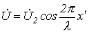 and
and 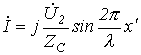 ,
,
whence, for the instantaneous values of voltage and current, we can write
 ; ; |
(19) |
 . . |
(20) |
These last equations are the equations of standing waves resulting from the superposition of forward and backward waves of equal amplitude.
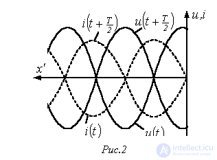
At OC, in accordance with (19) and (20), at points with coordinates  , where
  is an integer, voltage maxima occur, called antinodes, and current zeros occur, called nodes. At points with coordinates
 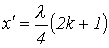 the antinodes and nodes of voltage and current are interchanged (see Fig. 2). Thus, the nodes and antinodes are stationary, and the antinodes of one variable coincide with the nodes of the other, and vice versa.
At SC, on the basis of equations (17) and (18)
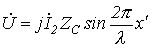 and
and 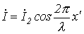 ,
,
whence, for the instantaneous values, we can write
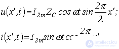
i.e., in this case too the voltage and current are standing waves, and, compared with the OC mode, the antinodes and nodes of voltage and current, respectively, are interchanged.
Since the power at the nodes is identically zero, standing waves do not participate in transmitting energy along the line. Only traveling waves transmit it. The more the load differs from the matched condition, the more pronounced the backward, and consequently standing, waves become. In the limiting cases of OC and SC considered, only standing waves are present, and the power at the load is zero.
References
Review questions and problems
Answer:  ;
; 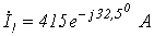 ;
;  .
.
Answer:  .
.
Answer:  ;
;  ;
;  ;
;  ;
;  .
.
Answer:  .
.
Answer:  .
.
 , if
, if 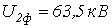 ,
, 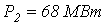 ,
,  . The line parameters per phase:
  ,
,  ,
,  ,
,  . Determine the efficiency of the line.
 at a frequency of 100 MHz. The characteristic impedance is
  .
. , a wave propagation speed of
 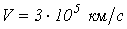 , and an attenuation of 1.5 Np per 100 km. Determine the primary parameters of the line, and also its efficiency for a length of
  and a load equal to the characteristic impedance.
 ,
, 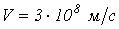 . At the end of the line
  . Find
  at a distance of 1 m from the end of the line.
 is open-circuited at the end.
  , at the beginning of the line
  . Find
  at the middle of the line.
Comments