
Lecture
Alternating current did not find practical application for a long time. This was because the first electrical energy generators produced direct current, which fully satisfied the technological processes of electrochemistry, and DC motors have good control characteristics. However, as production developed, direct current increasingly failed to satisfy the growing requirements of economical power supply. Alternating current made it possible to efficiently subdivide electrical energy and change voltage levels using transformers. It became possible to generate electric power at large power plants with subsequent economical distribution to consumers, and the radius of power supply increased.
At present, the central generation and distribution of electrical energy is carried out mainly using alternating current. Circuits with changing – alternating – currents have a number of distinctive features compared with direct-current circuits. Alternating currents and voltages give rise to alternating electric and magnetic fields. As a result of the variation of these fields, the phenomena of self-induction and mutual induction arise in the circuits, which have a very substantial effect on the processes occurring in circuits, complicating their analysis.
Alternating current (voltage, EMF, etc.) is a current (voltage, EMF, etc.) that varies with time. Currents whose values repeat at equal time intervals in the same sequence are called periodic, and the smallest time interval over which these repetitions are observed is called the period T. For a periodic current we have
 , , |
(1) |
The quantity that is the reciprocal of the period is the frequency, measured in hertz (Hz):
 , , |
(2) |
The range of frequencies used in engineering: from ultra-low frequencies (0.01¸10 Hz – used in automatic control systems, in analog computing) – to ultra-high frequencies (3000 ¸ 300000 MHz – millimeter waves: radar, radio astronomy). In the Russian Federation, the industrial (mains) frequency is f = 50Hz.
The instantaneous value of a varying quantity is a function of time. It is customarily denoted by a lowercase letter:
i - instantaneous value of current  ;
;
u – instantaneous value of voltage  ;
;
e - instantaneous value of EMF  ;
;
p- instantaneous value of power  .
.
The largest instantaneous value of a varying quantity over a period is called the amplitude (it is customarily denoted by a capital letter with the subscript m).
 - amplitude of the current;
 - amplitude of the voltage;
 - amplitude of the EMF.
RMS value of alternating current
The value of a periodic current equal to the value of a direct current that, over the time of one period, produces the same thermal or electrodynamic effect as the periodic current is called the root-mean-square (RMS) value of the periodic current:
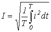 , , |
(3) |
The RMS values of EMF and voltage are defined analogously.
Sinusoidally varying current
Of all the possible forms of periodic currents, the sinusoidal current has become the most widespread. Compared with other types of current, sinusoidal current has the advantage that, in general, it allows the most economical generation, transmission, distribution, and use of electrical energy. Only when sinusoidal current is used is it possible to keep the shapes of the voltage and current curves unchanged at all points of a complex linear circuit. The theory of sinusoidal current is the key to understanding the theory of other types of circuits.
Representation of sinusoidal EMFs, voltages
and currents on the plane of Cartesian coordinates
Sinusoidal currents and voltages can be represented graphically, written by means of equations with trigonometric functions, represented as vectors on the Cartesian plane, or represented by complex numbers.
The graphs of two sinusoidal EMFs e1 and e2 shown in Fig. 1, 2 correspond to the equations:
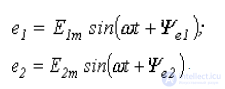
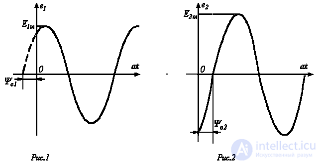
The values of the arguments of the sinusoidal functions  and
and  are called the phases of the sinusoids, and the value of the phase at the initial instant of time (t=0):
  and
and  is called the initial phase (
 ).
).
The quantity  , which characterizes the rate of change of the phase angle, is called the angular frequency. Since, over the time of one period T, the phase angle of the sinusoid changes by
  rad, the angular frequency is
 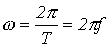 , where f– is the frequency.
When two sinusoidal quantities of the same frequency are considered together, the difference of their phase angles, equal to the difference of their initial phases, is called the phase shift angle.
For the sinusoidal EMFs e1 and e2 the phase shift angle is:
 .
.
Vector representation of sinusoidally
varying quantities
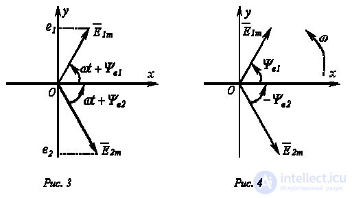
On the Cartesian plane, vectors equal in magnitude to the amplitude values of the sinusoidal quantities are drawn from the origin, and these vectors are rotated counterclockwise (in circuit theory this direction is taken as positive) with an angular frequency equal to w. The phase angle during rotation is measured from the positive half-axis of abscissas. The projections of the rotating vectors onto the ordinate axis are equal to the instantaneous values of the EMFs e1 and e2 (Fig. 3). The set of vectors representing sinusoidally varying EMFs, voltages, and currents is called a phasor (vector) diagram. When constructing phasor diagrams, it is convenient to place the vectors for the initial instant of time (t=0), which follows from the equality of the angular frequencies of the sinusoidal quantities and is equivalent to the Cartesian coordinate system itself rotating counterclockwise at speed w. Thus, in this coordinate system the vectors are stationary (Fig. 4). Phasor diagrams have found wide application in the analysis of sinusoidal-current circuits. Their use makes circuit calculation more illustrative and simple. This simplification consists in the fact that the addition and subtraction of instantaneous values of quantities can be replaced by the addition and subtraction of the corresponding vectors.
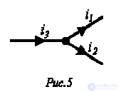
Suppose, for example, that at a branch point of a circuit (Fig. 5) the total current  is equal to the sum of the currents
  and
and  of two branches:
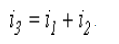 .
.
Each of these currents is sinusoidal and can be represented by the equation
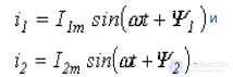
The resulting current will also be sinusoidal:
 .
.
Determining the amplitude and initial phase
  of this current by means of the corresponding trigonometric transformations turns out to be rather cumbersome and not very illustrative, especially when a large number of sinusoidal quantities are being summed. This is accomplished much more simply with the help of a phasor diagram.
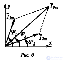
Fig. 6 shows the initial positions of the current vectors, whose projections onto the ordinate axis give the instantaneous values of the currents for t=0. As these vectors rotate at the same angular velocity w their relative arrangement does not change, and the phase-shift angle between them remains equal to 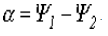 .
.
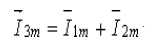
Since the algebraic sum of the projections of the vectors onto the ordinate axis equals the instantaneous value of the total current, the vector of the total current equals the geometric sum of the current vectors:
 .
.
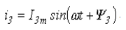
Constructing a phasor diagram to scale makes it possible to determine the values of and from the diagram, after which the solution for the instantaneous value can be written by formally accounting for the angular frequency:
 .
.
Representation of sinusoidal EMFs, voltages and currents by complex numbers
Geometric operations with vectors can be replaced by algebraic operations with complex numbers, which substantially increases the accuracy of the results obtained.
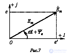
Each vector on the complex plane corresponds to a specific complex number, which can be written in:
exponential 
trigonometric  or
or
algebraic  forms.
For example, the EMF  , represented in Fig. 7 by a rotating vector, corresponds to the complex number
 .
.
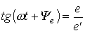
The phase angle  is determined from the projections of the vector onto the “+1” and “+j” axes of the coordinate system, as
 .
.
In accordance with the trigonometric form of notation, the imaginary component of the complex number determines the instantaneous value of the sinusoidally varying EMF:
 , , |
(4) |
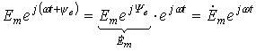
The complex number  is conveniently represented as the product of two complex numbers:
 , , |
(5) |
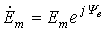
The parameter  , corresponding to the position of the vector for t=0 (or on the complex plane rotating at speed w ), is called the complex amplitude:
  , and the parameter
  is the complex instantaneous value.
The parameter  is the rotation operator of the vector through the angle wt relative to the initial position of the vector.
In general, multiplying a vector by the rotation operator  is its rotation relative to the initial position through the angle ±a.
Consequently, the instantaneous value of the sinusoidal quantity equals the imaginary part, without the sign “j”, of the product of the amplitude complex and the rotation operator :
 .
.
The transition from one form of writing a sinusoidal quantity to another is carried out by means of Euler's formula:
 , , |
(6) |
If, for example, the complex amplitude of the voltage is given as a complex number in algebraic form:
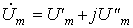 ,
,
then, to write it in exponential form, it is necessary to find the initial phase  , i.e., the angle that the vector
  forms with the positive half-axis +1:
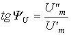 .
.
Then the instantaneous value of the voltage:
 ,
,
where  .
.
In writing the expression, for definiteness it was assumed that  , i.e., that the representative vector lies in the first or fourth quadrant. If
  , then for
  (second quadrant)
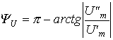 , , |
(7) |
and for  (third quadrant)
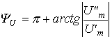 |
(8) |
or
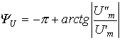 |
(9) |
If the instantaneous value of the current is given in the form  , the complex amplitude is first written in exponential form, and then (if necessary) converted to algebraic form by means of Euler's formula:
 .
.
It should be noted that for addition and subtraction of complex numbers, the algebraic form of their notation should be used, while for multiplication and division the exponential form is convenient.
Thus, the use of complex numbers makes it possible to move from geometric operations on vectors to algebraic operations on complex numbers. For example, when determining the complex amplitude of the resulting current from Fig. 5, we obtain:

where  ;
;
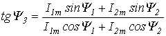 .
.
RMS value of sinusoidal EMFs, voltages, and currents
In accordance with expression (3), for the RMS value of a sinusoidal current we write:
 .
.
A similar result can be obtained for sinusoidal EMFs and voltages. Thus, the RMS values of sinusoidal current, EMF, and voltage are smaller than their amplitude values by a factor of  :
:
 . . |
(10) |
Since, as will be shown later, the energy calculation of AC circuits is usually carried out using RMS values of quantities, by analogy with the above we introduce the concept of the RMS-value complex
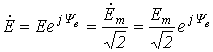 .
.
1. What is the practical significance of representing sinusoidal quantities by means of vectors?
2. What is the practical significance of representing sinusoidal quantities using complex numbers?
3. What are the advantages of representing sinusoidal quantities by complex numbers compared with their vector representation?
4. For the given sinusoidal functions of EMF and current  , write the corresponding amplitude and RMS-value complexes, as well as the instantaneous-value complexes.
5. In Fig. 5, 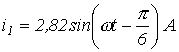 , and
, and 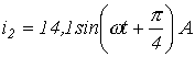 . Determine .
Answer:  .
.

Comments