
Lecture
Electromagnetic processes taking place in electrical engineering devices are, as a rule, fairly complex. However, in many cases their basic characteristics can be described using such integral concepts as voltage, current, and electromotive force (EMF). With this approach, a set of electrical engineering devices consisting of appropriately connected sources and receivers of electrical energy, intended for the generation, transmission, distribution and (or) conversion of electrical energy and/or information, is regarded as an electric circuit. An electric circuit consists of separate parts (objects) that perform specific functions and are called circuit elements. The principal elements of a circuit are sources and receivers of electrical energy (signals). Electrical engineering devices that produce electrical energy are called generators or sources of electrical energy, while devices that consume it are called receivers (loads, consumers) of electrical energy.
For each circuit element a certain number of terminals (poles) can be identified, by means of which it is connected to other elements. A distinction is made between two-terminal and multi-terminal elements. Two-terminal elements have two terminals. These include energy sources (except controlled and polyphase ones), resistors, inductors, and capacitors. Multi-terminal elements are, for example, triodes, transformers, amplifiers, etc.
All elements of an electric circuit can conventionally be divided into active and passive. An element is called active if it contains a source of electrical energy within its structure. Passive elements are those in which energy is dissipated (resistors) or stored (inductors and capacitors). The principal characteristics of circuit elements are their voltage-current, weber-ampere, and coulomb-voltage characteristics, described by differential and/or algebraic equations. If the elements are described by linear differential or algebraic equations, they are called linear; otherwise they belong to the class of nonlinear elements. Strictly speaking, all elements are nonlinear. The possibility of treating them as linear – which substantially simplifies the mathematical description and analysis of the processes – is determined by the range of variation of their characteristic variables and frequencies. The coefficients relating the variables, their derivatives, and their integrals in these equations are called the parameters of the element.
If the parameters of an element are not functions of the spatial coordinates that determine its geometric dimensions, it is called a lumped-parameter element. If an element is described by equations that include spatial variables, it belongs to the class of distributed-parameter elements. A classic example of the latter is an electric power transmission line (a long line).
Circuits containing only linear elements are called linear. The presence of even one nonlinear element in a circuit places it in the class of nonlinear circuits.
Let us consider the passive elements of a circuit, their basic characteristics and parameters.
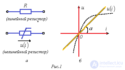
The conventional graphic symbol of a resistor is shown in Fig. 1,a. A resistor is a passive element characterized by resistance. The latter is determined by the geometric dimensions of the body and the properties of the material: the resistivity r (Ohm´m) or its reciprocal – the conductivity  (S/m).
In the simplest case of a conductor of length  and cross-section S, its resistance is determined by the expression
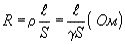 .
.
In the general case, determining the resistance requires calculating the field in the conducting medium that separates the two electrodes.
The main characteristic of a resistive element is the relationship  (or
(or  ), called the current-voltage characteristic (CVC). If the relationship is a straight line passing through the origin (see Fig. 1,b), the resistor is called linear and is described by the relation

or
 ,
,
where  is the conductance. In this case R = const.
A nonlinear resistive element, whose CVC is nonlinear (Fig. 1,b), is characterized by several parameters, as will be shown in the block of lectures devoted to nonlinear circuits. In particular, an inertialess resistor is assigned a static resistance  and a differential resistance
  .
.
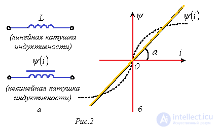
The conventional graphic symbol of an inductor is shown in Fig. 2,a. An inductor is a passive element characterized by inductance. To calculate the inductance of a coil, the magnetic field it creates must be calculated.
Inductance is defined as the ratio of the flux linkage to the current flowing through the turns of the coil,
 .
.
In turn, the flux linkage equals the sum of the products of the flux threading the turns and the number of those turns 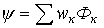 , where
  .
.
The main characteristic of an inductor is the relationship  , called the weber-ampere characteristic. For linear inductors, the relationship is a straight line passing through the origin (see Fig. 2,b); in this case
 .
.
The nonlinear properties of an inductor (see curve in Fig. 2,b) are determined by the presence of a ferromagnetic core, for which the relationship 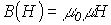 between magnetic flux density and field strength is nonlinear. Neglecting the phenomenon of magnetic hysteresis, a nonlinear inductor is characterized by a static inductance
  and a differential inductance
  .
.
The conventional graphic symbol of a capacitor is shown in Fig. 3,a.
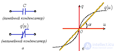
A capacitor is a passive element characterized by capacitance. To calculate the latter, the electric field in the capacitor must be calculated. Capacitance is defined as the ratio of the charge q on the capacitor plates to the voltage u between them

and depends on the geometry of the plates and the properties of the dielectric between them. Most dielectrics used in practice are linear, i.e., their relative permittivity = const. In this case the relationship
  is a straight line passing through the origin (see Fig. 3,b), and
 .
.
For nonlinear dielectrics (ferroelectrics), the permittivity is a function of the field strength, which causes the relationship to be nonlinear (Fig. 3,b). In this case, neglecting the phenomenon of electric hysteresis, a nonlinear capacitor is characterized by a static  and differential
  capacitance.
Equivalent circuits of electrical energy sources
The properties of an electrical energy source are described by the CVC  , called the external characteristic of the source. Further in this section, for simplicity of analysis and mathematical description, we will consider DC voltage (current) sources. However, all the relationships, concepts, and equivalent circuits obtained in doing so apply equally to AC sources. The CVC of a source can be determined experimentally using the circuit shown in Fig. 4,a. Here voltmeter V measures the voltage at terminals 1-2 of source S, while ammeter A measures the current I drawn from it, whose value can be varied by means of a variable load resistor (rheostat) RN.
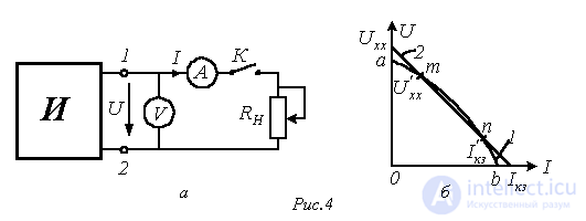
In the general case, the CVC of a source is nonlinear (curve 1 in Fig. 4,b). It has two characteristic points, corresponding to:
a – the no-load (open-circuit) mode 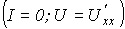 ;
;
b – the short-circuit mode 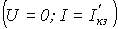 .
.
For most sources, the short-circuit mode (and sometimes the no-load mode) is not permissible. The currents and voltages of a source can generally vary within certain limits, bounded above by values corresponding to the rated mode (the mode at which the manufacturer guarantees the best operating conditions in terms of efficiency and service life). This makes it possible, in a number of cases, to simplify calculations by approximating the nonlinear CVC on the working segment m-n (see Fig. 4,b) by a straight line whose position is determined by the working ranges of variation of voltage and current. It should be noted that many sources (galvanic cells, batteries) have linear CVCs.
Line 2 in Fig. 4,b is described by the linear equation
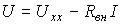 , , |
(1) |
where  is the voltage at the source terminals with the load disconnected (with switch K open in the circuit of Fig. 4,a);
 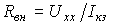 is the internal resistance of the source.
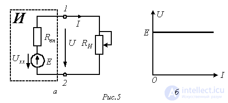
Equation (1) makes it possible to construct a series equivalent circuit for the source (see Fig. 5,a). In this circuit, the symbol E denotes an element called an ideal EMF source. The voltage at the terminals of this element 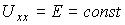 does not depend on the source current, and therefore corresponds to the CVC in Fig. 5,b. From (1), for such a source
  . Note that the directions of the EMF and of the voltage at the source terminals are opposite.
If the CVC of a source is linear, then to determine the parameters of its equivalent circuit it is sufficient to take voltage and current measurements for any two of its operating modes.
There is also a parallel equivalent circuit for a source. To derive it, divide both sides of relation (1) by  . This gives
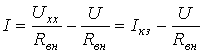
or
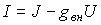 , , |
(2) |
where  ;
;  is the internal conductance of the source.
Equation (2) corresponds to the source equivalent circuit in Fig. 6,a.
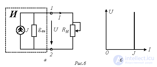
In this circuit, the symbol J denotes an element called an ideal current source. The current in the branch containing this element equals and does not depend on the voltage at the source terminals, and therefore corresponds to the CVC in Fig. 6,b. On this basis, taking (2) into account, for such a source  , i.e., its internal resistance
  .
.
Note that, from a computational standpoint, provided the condition  holds, the series and parallel equivalent circuits of the source are equivalent. However, in terms of energy they differ, since in the no-load mode the power for the series equivalent circuit equals zero, whereas for the parallel one it does not.
In addition to the operating modes noted above, the matched mode is of considerable practical importance, in which the load RN draws maximum power from the source
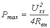 , , |
(3) |
The condition for this mode is
 , , |
(4) |
In conclusion, note that, in accordance with the CVCs in Fig. 5,b and 6,b, ideal EMF and current sources are sources of infinitely large power.
Answer: L=0.1 H; WM=40 J.
Answer: C=0.5 uF; WE=0.04 J.
Answer: 
Answer: 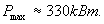
explain the graphs 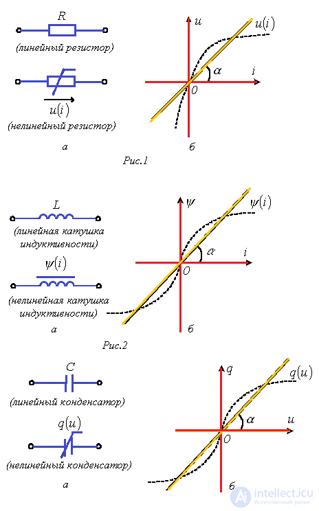

Comments