34. Nonlinear AC Circuits in Steady-State Modes

AC circuits in steady-state operation may contain nonlinear elements such as diodes, transistors, thyristors, and other semiconductor devices. These elements can change their characteristics depending on the voltage or current flowing through them, which leads to nonlinear behavior of the circuit as a whole.

Features of nonlinear circuits under alternating currents

The most significant feature of calculating nonlinear circuits under alternating currents is the need to account, in the general case, for the dynamic properties of nonlinear elements, i.e., their analysis should be carried out on the basis of dynamic volt-ampere, weber-ampere, and coulomb-volt characteristics.

If a nonlinear element is inertialess, its characteristics in dynamic and static modes coincide, which significantly simplifies the calculation. In practice, however, ideally inertialess elements do not exist. Whether a nonlinear element can be classified as inertialess is determined by the rate of change of the input action: if the period T of the alternating action is sufficiently small compared with the time constant , characterizing the dynamic properties of the nonlinear element, the latter is treated as inertialess; if this condition is not met, the inertial properties of the nonlinear element must be taken into account.

The most significant feature of calculating nonlinear circuits under alternating currents is the need to account, in the general case, for the dynamic properties of nonlinear elements, i.e., their analysis should be carried out on the basis of dynamic volt-ampere, weber-ampere, and coulomb-volt characteristics.

If a nonlinear element is inertialess, its characteristics in dynamic and static modes coincide, which significantly simplifies the calculation. In practice, however, ideally inertialess elements do not exist. Whether a nonlinear element can be classified as inertialess is determined by the rate of change of the input action: if the period T of the alternating action is sufficiently small compared with the time constant , characterizing the dynamic properties of the nonlinear element, the latter is treated as inertialess; if this condition is not met, the inertial properties of the nonlinear element must be taken into account.

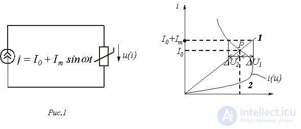
As an example, we can consider the circuit in Fig. 1 with a nonlinear resistor (thermistor) having a volt-ampere characteristic (VAC) shown in Fig. 2, and characterized by a heating time constant .

If , the representative point moves along straight line 1, and the nonlinear resistor is characterized by the resistance . For the representative point moves along curve 2, and the properties of the nonlinear resistor are determined by the resistance . When the heating time constant t_NR is of the same order as T, the relationships between the variable components of voltage and current become more complex, giving rise to a phase shift between them.

Another important feature of nonlinear elements in an AC circuit is that they cause the appearance of higher harmonics even when the circuit contains only sinusoidal voltage and/or current sources. This principle underlies, for example, a number of frequency multipliers, as well as current or voltage waveform converters.

Basic types of characteristics of nonlinear elements in AC circuits

Using the dynamic characteristics of nonlinear elements makes it possible to calculate nonlinear circuits in terms of the instantaneous values of the variables, i.e., to carry out, in principle, the most accurate and complete analysis. However, in a number of cases such a calculation can turn out to be fairly labor-intensive or excessive in its depth of detail. Therefore, depending on the purpose of the problem being solved and the required accuracy of the results, besides the dynamic characteristic, nonlinear characteristics for the first harmonics and for rms values may also be used (see Table 1).

Table 1. Definitions of the basic types of characteristics of nonlinear elements

Graphical calculation methods

Graphical calculation methods make it possible to analyze nonlinear AC circuits for particular parameter values using the characteristics of nonlinear elements for instantaneous values, first harmonics, and rms values (see Table 1).

Graphical method using characteristics for instantaneous values

In general, the procedure for analyzing a nonlinear circuit by this method includes the following steps:

• -based on physical considerations, the law of variation (if not given) of one of the quantities defining the characteristic of the nonlinear element is found;
• -using the nonlinear characteristic and the known law of variation of the quantity , the curve is determined by graphical construction (or vice versa);
• -using the resulting relationship , the rest of the (linear) part of the circuit is analyzed.

As an example, let us construct, for a sinusoidal EMF , the current curve in the circuit of Fig. 3, whose diode VAC is shown in Fig. 4.

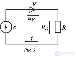
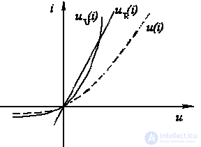
Fig. 4

Solution

1. We construct the resulting VAC of the circuit (see Fig. 4) according to the relationship

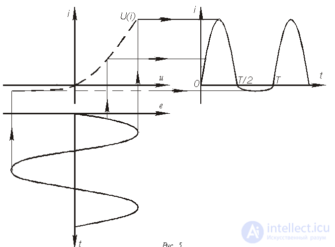
2. By finding, for various values of , the corresponding current values using the resulting curve, we plot point by point (see Fig. 5) the curve of the required relationship .

The following comment should be made regarding the result obtained. Using the VAC of an ideal valve (no reverse current, and zero voltage drop across the diode in the conducting direction) in the analysis of such circuits is correct for sufficiently large amplitudes of the voltage applied to the diode, for which the forward current through the valve significantly exceeds its reverse current, so that the latter can be neglected. When the voltage values decrease and these currents become comparable in magnitude, the VAC of a real diode, shown in Fig. 4 and accounting for the reverse current, should be used.

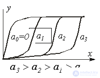
One of the most important elements in AC circuits is a coil with a ferromagnetic core. In general, the curve has the shape of a hysteresis loop, but since devices operating under alternating voltage use magnetic materials with a narrow hysteresis loop, in most practical cases it is acceptable to use the basic (or initial) magnetization curve in calculations.

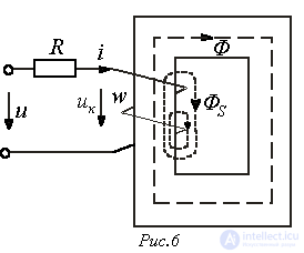
A schematic representation of a nonlinear inductor is shown in Fig. 6. Here – is the main flux, closing through the core, and - is the leakage flux, to which, in a first approximation, the leakage flux linkage can be assigned, where the leakage inductance is due to the flux traveling part of its path through air.

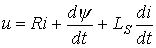
For the circuit in Fig. 6, the following equation holds

,

(1)

where .

In general, because of the nonlinearity of the relationship , it is fairly difficult to determine the non-sinusoidal relationships and from (1). At the same time, for real inductors, the voltage drop and the EMF due to the leakage fluxes can often be neglected because of their small magnitude. In this case, from (1) we obtain , from which

,

where is the constant of integration.

Since the characteristic of the coil (see Fig. 7) is symmetric about the origin, and the voltage is symmetric about the abscissa (the time axis), the curve must also be symmetric about the latter, from which it follows that .

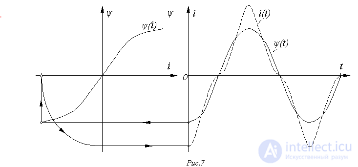
By finding, for various values of , the corresponding current values using the curve , we plot point by point (see Fig. 7) the curve of the relationship .

Analysis of the result obtained allows an important conclusion to be drawn: for a sinusoidal flux waveform, the voltage across the coil is sinusoidal, while the current flowing through it has a clearly non-sinusoidal shape. Similarly, it can be shown that for a sinusoidal current, the flux linked with the coil and the voltage across it are non-sinusoidal.

For the average value of the voltage induced by the flux, we can write

.

(2)

Multiplying (2) by the form factor, we obtain the expression for the rms value of the voltage

In particular, if the voltage and the flux are sinusoidal, then

.

Relation (2) is very important: by measuring the average value of the voltage induced by the flux, equation (2) can be used to determine the amplitudes of the flux and the flux density for any degree of nonlinearity of the coil.

The curve is constructed similarly for a sinusoidal flux and a given relationship in the form of a hysteresis loop. In this case, it should be remembered that the operating point moves along the loop counterclockwise (see Fig. 8).

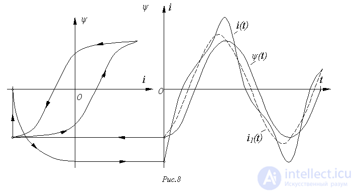
The following important comment should be made about the result obtained. Expanding the resulting curve in a Fourier series shows that the first harmonic of the current (see curve in Fig. 8) leads the flux linkage in phase and, consequently, lags the sinusoidal voltage on the coil in phase by an angle less than 90°. This indicates ( ) that the coil consumes active power, expended on remagnetizing the core and determined by the area of the hysteresis loop.

Review questions and problems

Answer: .

1. What are the features of nonlinear AC circuits?
2. What types of characteristics are used in AC circuits to describe nonlinear elements?
3. In what cases is it acceptable to use the ideal VAC of valves in calculations?
4. Why can the leakage flux linkage of a coil not be represented as the product of its number of turns and the leakage flux?
5. How can the amplitude of the magnetic flux density linked with a coil be determined indirectly?
6. Construct the curves and for a sinusoidal current in a nonlinear coil.
7. Why does the first harmonic of the expansion of the current curve , when the hysteresis loop is taken into account, lag the voltage by an angle less than 90°?
8. Determine the amplitude of the main working flux in the core of a nonlinear coil with cross-section , if, for a number of turns , the average value of the voltage due to the change in flux is ; frequency .