
Lecture
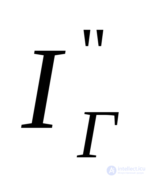
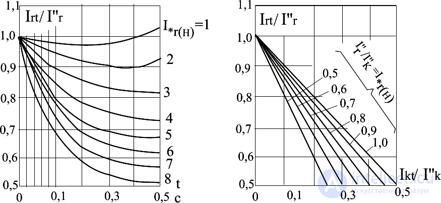
The typical curves method is based on using graphs of the time variation of the ratio of the rms value of the periodic component of the short-circuit current from generators at an arbitrary instant  to the initial value of this current
 (Fig. 5.6)

a)
b)
Fig.5.6. Typical curves of the time variation of the short-circuit current of a synchronous machine (with power up to and including 800 MW) for different distances of the fault point
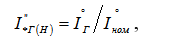
Usually, the electrical distance of the fault point from a synchronous machine is understood as the external resistance, reduced to the machine's rated power and rated voltage, that turns out to be connected to the machine as a result of the short circuit. However, such an estimate of distance is applicable only when the calculation circuit contains just one, or several synchronous machines, that are under identical conditions with respect to the fault point. A more convenient and universal quantity, which fully characterizes the distance of the fault point from a synchronous machine and can be determined in any circuit and for any number of power sources, is the ratio
 ,
,
where  – is the initial value of the short-circuit current of the generator (compensator);
 –is the rated current of the synchronous machine, reduced to the average rated voltage
 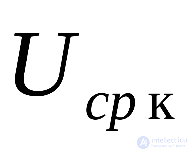 , of the voltage level at which the short circuit is being considered
This current is determined by the relation  , (5.2)
where  – is the rated power of the synchronous machine, MVA.
If short-circuit current calculations are carried out in per-unit values under arbitrarily chosen conditions, then  , (5.3)
where 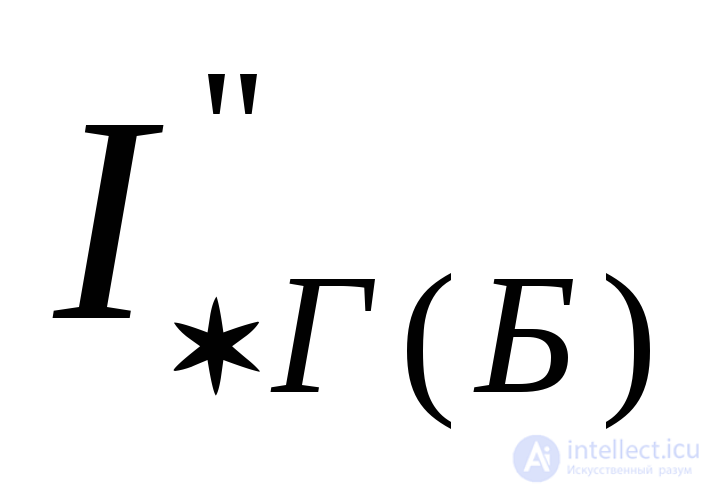 – is the current of the synchronous machine at the initial instant of the short circuit, expressed in per-unit values for arbitrarily chosen base conditions;
 –is the base power.
It is advisable to take  as the rated power of the machine, since in this case
 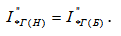 .
.
The typical curves make it possible to find the periodic component of the short-circuit current, for the time interval from 0 to 0,5 s, with an approximate account of the influence of the network load. The curves are valid for turbogenerators with power from 12,5 to 800 MW, hydrogenerators with power up to 500 MW, and for all large synchronous compensators.
The typical curves 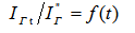 are constructed under the following conditions: the ceiling excitation for turbogenerators and synchronous compensators exceeds the rated value by a factor of 2, and for hydrogenerators– by a factor of 1,8; the time constant of the voltage rise on the field winding of the synchronous machine during forced excitation
 is taken as zero. The exception is the curve corresponding to
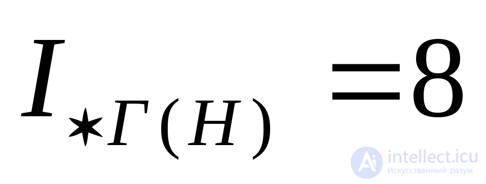 , in constructing which
 was taken equal to 0,25 s.
From the above method of constructing the typical curves, a simple procedure for their use follows.
If the calculation circuit contains a single generator (or several identical generators under the same conditions with respect to the fault point), it is advisable to carry out the short-circuit current calculation for instants of time up to 0,5 s in the following sequence:
1. An equivalent calculation circuit is set up to determine the initial value of the periodic component of the short-circuit current, in which the load branches are omitted, and the generator (compensator) is represented by the subtransient reactance 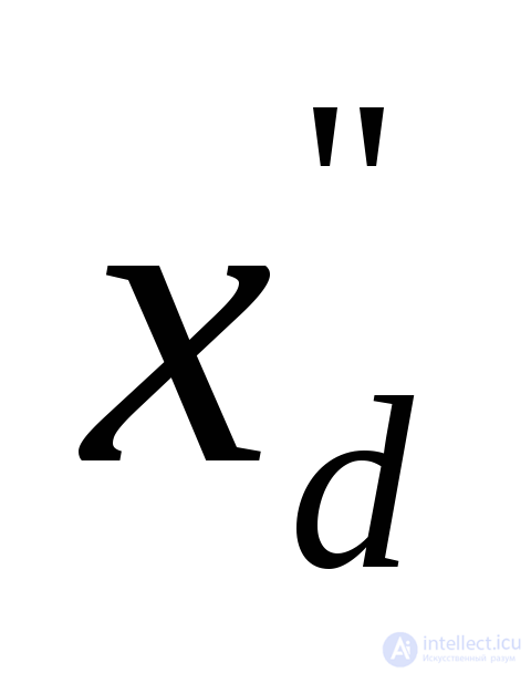 and the subtransient EMF
 , whose value (if not given in the initial data) can be determined from expression (5.1).
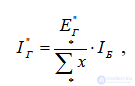
2. The total resistance of the equivalent circuit with respect to the short-circuit current 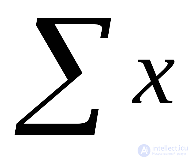 is determined, together with the initial value of the periodic component of the current at the point of a three-phase short circuit from the generator (or a group of identical generators)
 ,
,
where 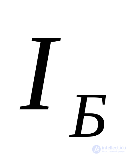 – is the base current of the voltage level at which the fault point is located.
3. Depending on the calculation method adopted (in named units or in per-unit values), the electrical distance of the fault point from the synchronous machine – 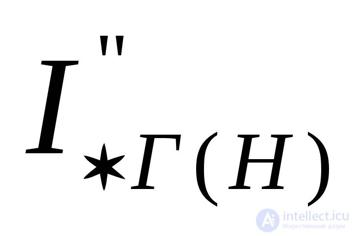 is determined from formulas (5.1) or (5.3). If there are several identical synchronous generators (compensators), the total power of all the generators must be substituted for
 in formulas (5.2) or (5.3).
4. From the curve 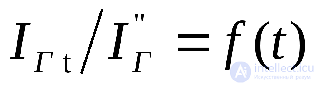 , corresponding to the found value
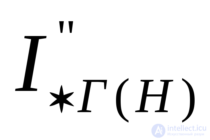 , the ratio of the short-circuit current at the required instant t to the initial value of the current, i.e.,
 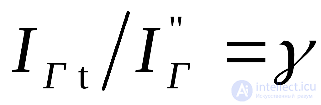 , is determined. If the value of the current
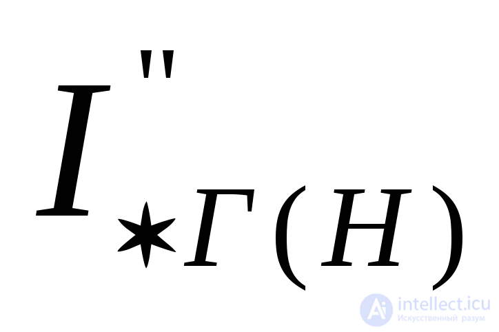 turns out to be a fractional number, it is rounded to the nearest whole number (if the difference between these numbers is small), or interpolation between the curves is performed.
5. From the found ratio 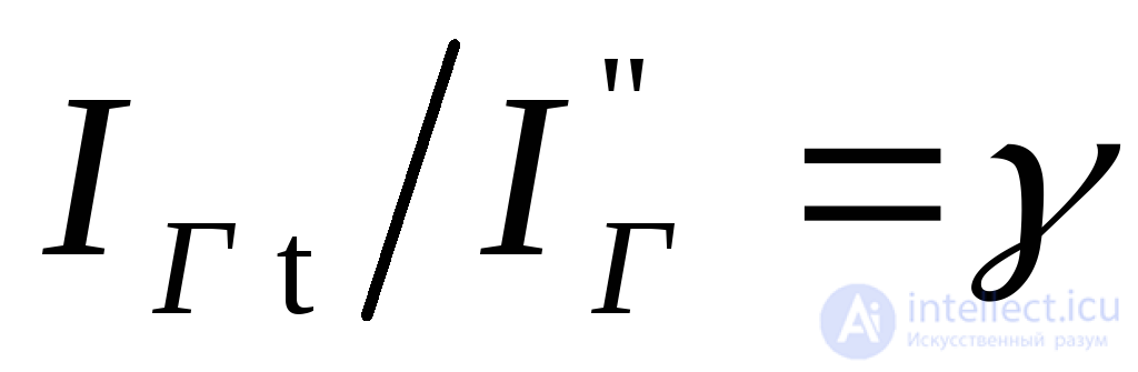 , the rms value of the periodic component of the short-circuit current from the generator (or group of generators) at instant t is determined.
The above short-circuit current calculation procedure also holds when the circuit contains several synchronous generators (compensators), provided the short circuit is three-phase, so that the generating branches are not connected to the fault location by a common resistance, i.e., they turn out to be independent of one another.
In this case, the subtransient EMFs of the different generators (compensators) are found, the total resistances and the initial values of the periodic component of the short-circuit currents of the individual branches are determined, the per-unit values of the currents of the different generators (compensators)  are determined from formulas (5.1) or (5.3), and the ratios
  are found from the corresponding typical curves. The currents
 are then found in named units, and the total current at the fault location is determined.
If the circuit has several finite-power sources at different electrical distances from the fault point, as well as a constant-voltage system, it is advisable to divide all the sources into two groups. Into one of them, include all the synchronous generators (compensators) located close to the fault point (connected to the fault point directly through a single transformation stage), and into the other group – the sources that are significantly remote from the fault point, including the rest of the power system, replacing them with a single source with constant voltage at its busbars (hereinafter called the system), Fig. 5.7, 5.8.
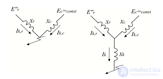
Fig.5.7. First calculation circuit Fig.5.8. Second calculation circuit
If the system is directly connected to the fault point, i.e., has no branches in common with the other sources (Fig. 5.7), then the rms value of the periodic component of the short-circuit current from the system should be found from the expression
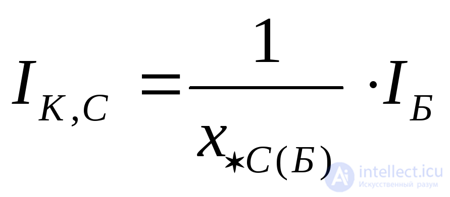 ,
,
where 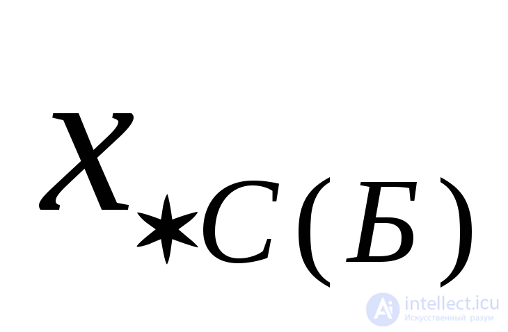 – total impedance up to the short-circuit point in per-unit values under the selected base conditions;
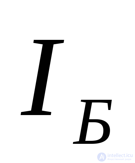 –base current of the voltage level at which the short-circuit point is located, kA.
In cases where the generator subject to individual accounting and the system are connected to the short-circuit point through a common impedance 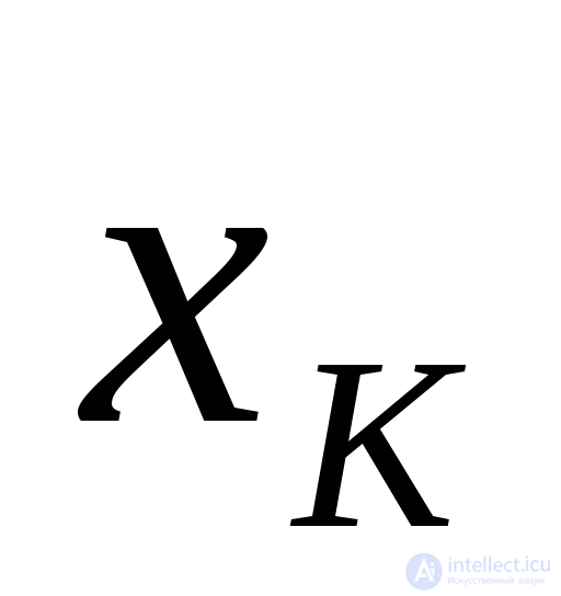 (Fig. 5.8), the change in the generator current over time causes a change in the current supplied from the system. The degree of current change at the short-circuit location at any moment of time t can be determined approximately from special curves
  , plotted for various ratios
 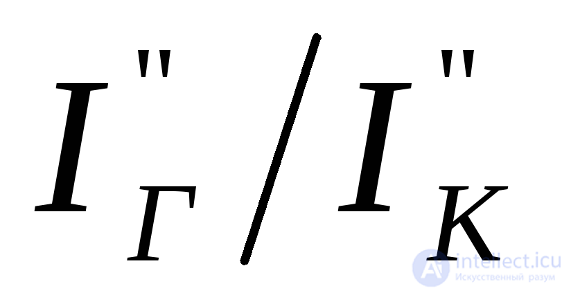 ranging from one to zero.
Example 5.4. Determine the three-phase short-circuit current at point K of the power plant, whose diagram is shown in Fig. 5.9, at time t = 0.2 s.
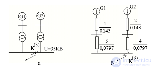
Fig. 5.9. For Example 5.4: a – original diagram; b – calculation diagram
The power plant has two identical synchronous generators rated at 37.5 MVA, cos = 0.8,
 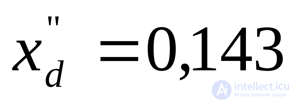 ,
, 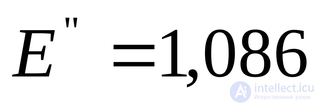 ; transformer parameters:
 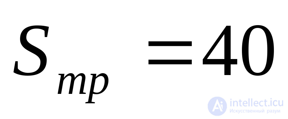 MVA;
MVA;
Solution:
The impedances of the elements of the power plant's equivalent circuit (Fig. 5.9, b) in per-unit values at 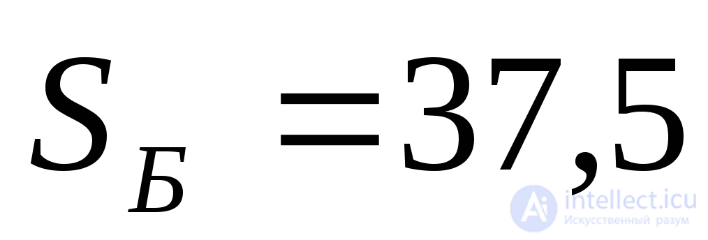 MVA,
MVA,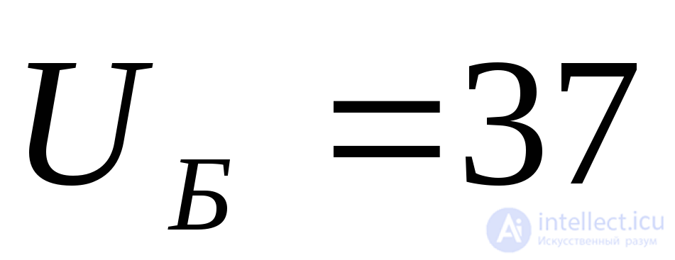 kV and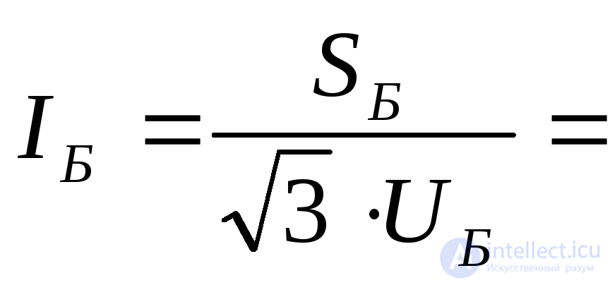
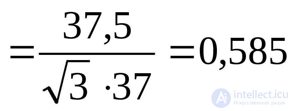 kA:
kA:

Rated current of each generator:
 .
.
Both generators are under identical conditions relative to the short-circuit point. Therefore, we treat them as a single equivalent generator with a resultant impedance 
Initial current produced by the equivalent generator during a three-phase short circuit:  .
.
Ratio of the equivalent generator's three-phase short-circuit current to the rated current of the individual generators:
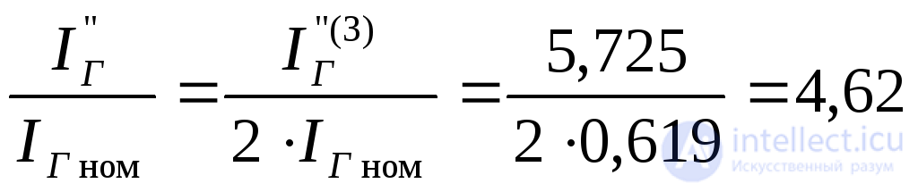 .
.
+From the curves (Fig. 5.6) for t = 0.2 s we find 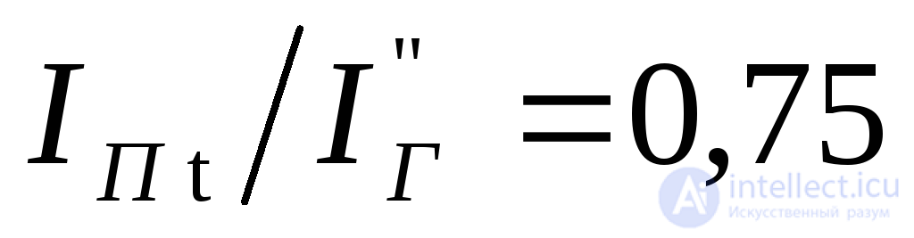 . The three-phase short-circuit current at point (K) produced by the equivalent generator at time t = 0.2 s.
 .
.
When calculating the short-circuit current in a network with voltage below 1000 V (Fig. 5.10), it can be assumed that the voltage on the high-voltage busbars (6-20 kV) of the step-down transformer remains unchanged ( ), provided the condition
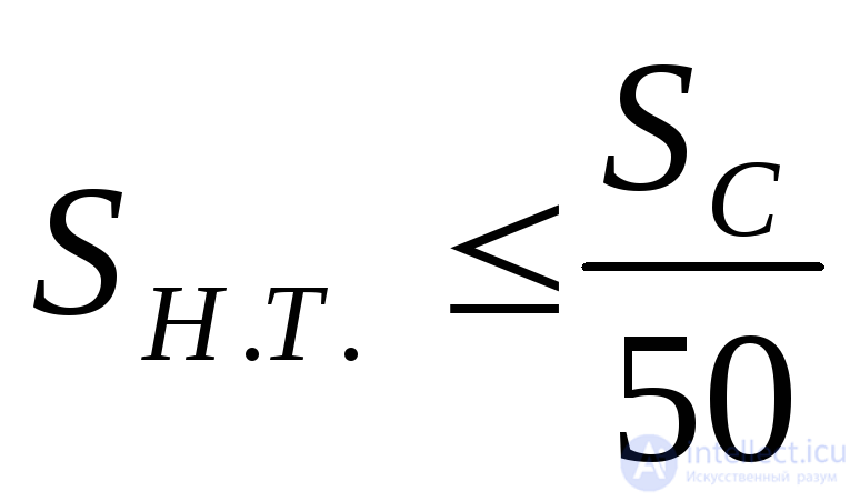 is satisfied,
where  - rated power of the step-down transformer;
 - installed generating capacity.
When calculating short-circuit currents in networks with voltage below 1000 V, an equivalent circuit is compiled that accounts for both the reactive and resistive impedances of the elements: the step-down transformer, current transformers, maximum-current relay coils of protective devices, cable and overhead lines, busways; and the resistances of transition contacts (switches, circuit breakers), etc.
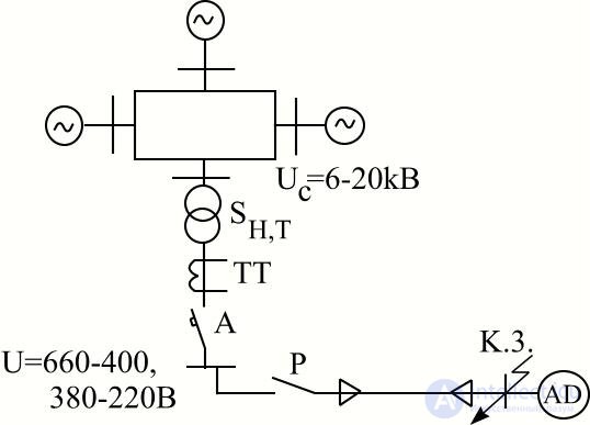
Fig. 5.10. Short circuit in networks up to 1000 volts
It is advisable to carry out the calculation in named units: power – kVA, current – A, voltage – V, resistance – MOhm (1 MOhm = 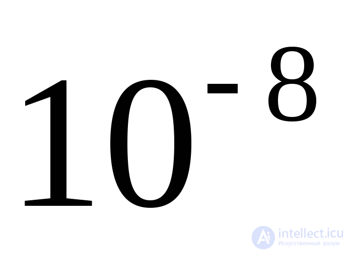 Ohm).
Ohm).
The equivalent circuit for the network (Fig. 5.10) is shown in Fig. 5.11.
The short-circuit current from the system is determined by the expression
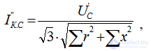 ,
,
where  - line voltage on the high-voltage busbars of the step-down transformer, referred to a voltage below 1000 V;
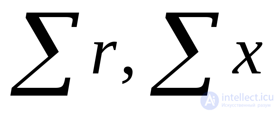 –total inductive and resistive impedances of the equivalent circuit from the transformer busbars to the short-circuit point.

Fig. 5.11. Equivalent circuit
The influence of induction motors connected directly to the short-circuit location on the values of 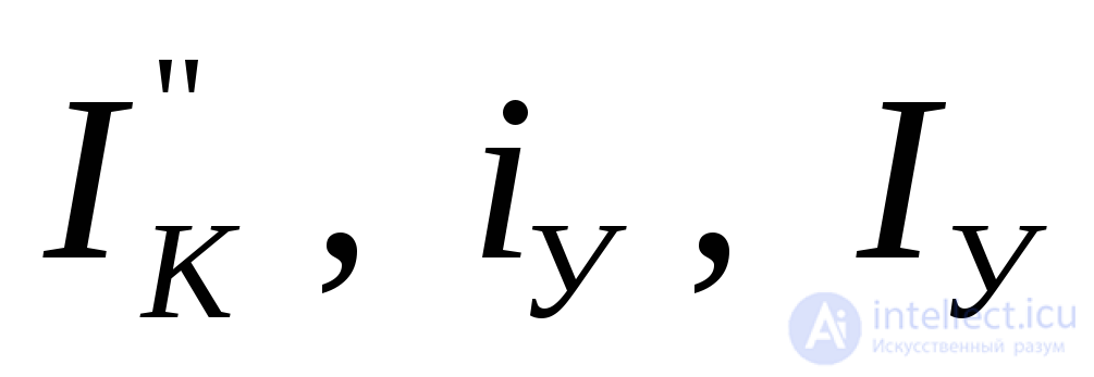 is recommended to be taken into account in all cases.
The feed current to the short-circuit location from induction motors is determined by the expression 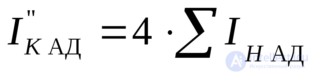 ,
,
where 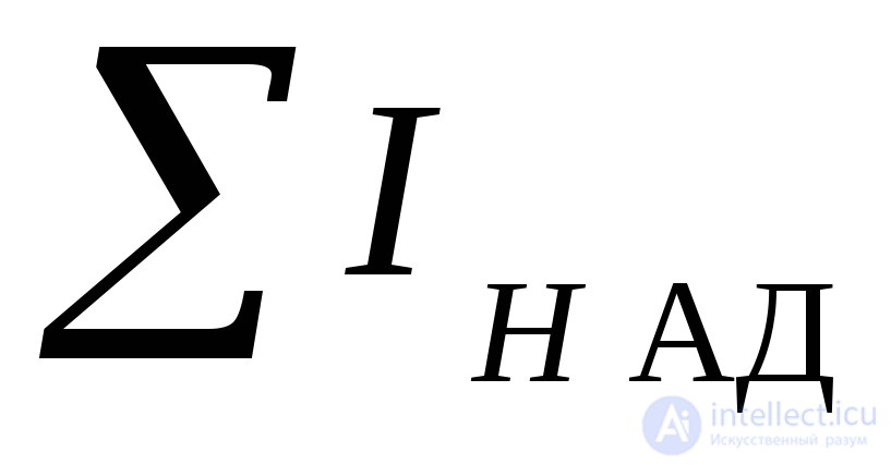 – value of the total rated current of the motors.
Then the total value of the short-circuit current is determined as the sum of the short-circuit currents from the system 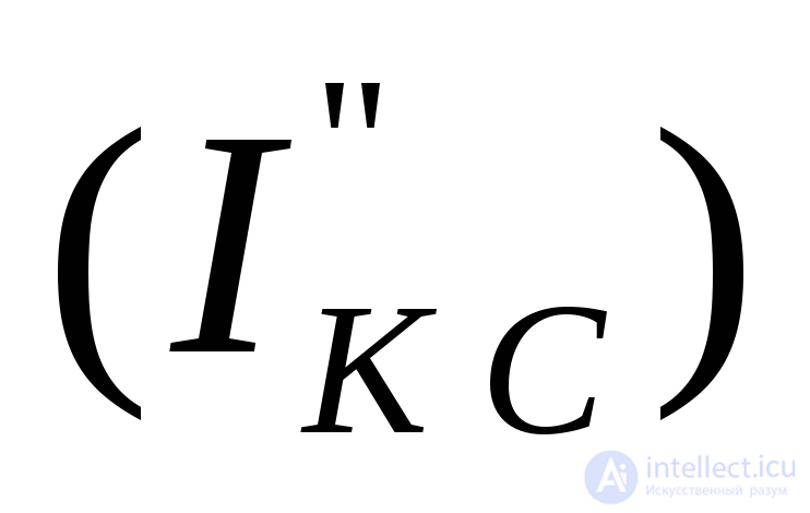 and from the motors
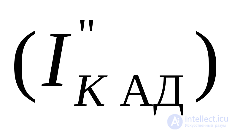 .
.
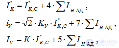
where  – coefficient determined from Fig. 5.12. depending on the ratio
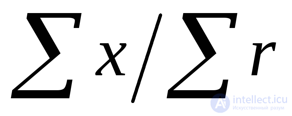 :
: 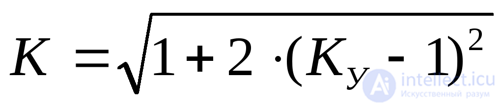 .
.
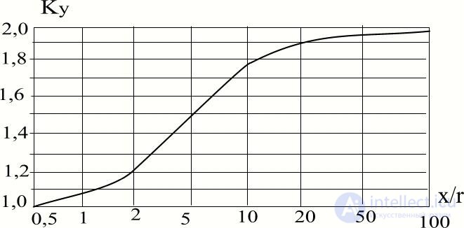
Fig. 5.12. Dependence of the surge (shock) coefficient on the ratio x/r

Comments