
Lecture
When solving electrical engineering problems, all substances are magnetically divided into two groups:
 );
); ).
).To concentrate the magnetic field and give it the desired configuration, certain parts of electrical devices are made of ferromagnetic materials. These parts are called magnetic cores. The magnetic flux is created by currents flowing through the windings of electrical devices, and less often by permanent magnets. The set of devices containing ferromagnetic bodies and forming a closed loop, along which the lines of magnetic induction close, is called a magnetic circuit.
The magnetic field is characterized by three vector quantities, which are given in Table 1.
Table 1. Vector quantities characterizing the magnetic field
|
Name, |
Definition |
|
Magnetic flux density vector T (tesla) |
A vector quantity characterizing the force exerted by the magnetic field on a current according to Ampere's law |
|
Magnetization vector A/m |
The magnetic moment per unit volume of a substance |
|
Magnetic field strength vector A/m |
where |
The main scalar quantities used in calculating magnetic circuits are given in Table 2.
Table 2. Main scalar quantities characterizing a magnetic circuit
|
Name, |
Definition |
|
Magnetic flux
Wb (weber) |
The flux of the magnetic flux density vector through the cross section
|
|
Magnetomotive (magnetizing) force MMF (F)
A |
|
|
Magnetic voltage
A |
The line integral of the magnetic field strength |
The properties of ferromagnetic materials are characterized by the dependence  of magnetic induction on magnetic field strength. Here a distinction is made between magnetization curves, which are single-valued dependences
  , and hysteresis loops, which are multi-valued dependences
  (see Fig. 1).
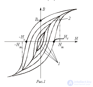
The basic concepts characterizing the dependences  are given in Table 3.
Table 3. Basic concepts characterizing the dependences 
|
Concept |
Definition |
|
Magnetic hysteresis |
The phenomenon of the lag of the change in magnetic induction B behind the change in magnetic field strength H |
|
Static hysteresis loop |
The dependence The area of the static hysteresis loop characterizes the losses due to magnetic hysteresis over one cycle of change of the magnetic field strength |
|
Initial magnetization curve |
The magnetization curve of a previously demagnetized ferromagnet (B=0;H=0) under a smooth change of the magnetic field strength H. It represents a single-valued dependence |
|
Basic magnetization curve |
The locus of the vertices of the magnetic hysteresis loops (see curve 2 in Fig. 1). It represents a single-valued dependence |
|
Limiting hysteresis loop (limit cycle) |
A symmetric hysteresis loop at the maximum possible saturation |
|
Coercive force |
The magnetic field strength Hc required to bring the magnetic induction in a previously magnetized ferromagnet to zero. In reference literature it is usually given for the limiting hysteresis loop |
|
Residual induction |
The value of the magnetic field induction Br at zero magnetic field strength. In reference literature it is usually given for the limit cycle |
Remagnetization of a ferromagnetic material involves the expenditure of energy on this process. As already noted, the area of the hysteresis loop characterizes the energy dissipated per unit volume of the ferromagnet during one remagnetization cycle. Depending on the magnitude of these losses, and accordingly on the shape of the hysteresis loop, ferromagnetic materials are divided into soft magnetic and hard magnetic materials. The former are characterized by a relatively narrow hysteresis loop and a steeply rising basic magnetization curve; the latter have a large hysteresis loop area and a gently rising basic magnetization curve.
Soft magnetic materials (electrical steels, iron-nickel alloys, ferrites) provide low core losses and are used in devices designed to operate under alternating magnetic flux (transformers, electric motors, etc.). Hard magnetic materials (carbon steels, tungsten alloys, etc.) are used to manufacture permanent magnets.
Static and differential magnetic permeability
Static magnetic permeability (in reference books, the initial and maximum values)
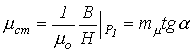 |
(1) |
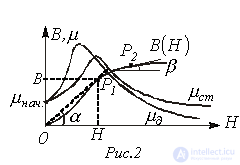
is determined from the basic magnetization curve and, owing to its nonlinearity, is not constant in magnitude (see Fig. 2).
The value  is determined by the tangent of the slope angle of the tangent line at the origin of the curve
  .
.
In addition to the static permeability, the concept of differential magnetic permeability is introduced, which establishes the relationship between infinitesimally small increments of induction and field strength
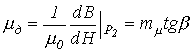 . . |
(2) |
The curves  and
and  have two common points: the initial point and the point corresponding to the maximum of
  (see Fig. 2).
When the hysteresis loop is taken into account, the static magnetic permeability defined by (1) loses its meaning. In this case the values of  are determined from the ascending branch of the loop for
  and from the descending branch for
  .
.
For an alternating magnetic flux, the concept of dynamic magnetic permeability is also introduced, defined by a relation analogous to (2), based on the dynamic characteristic.
The calculation of magnetic circuits is based on two laws (see Table 4).
Table 4. Basic laws of the magnetic circuit
|
Name |
Analytical expression of the law, |
|
Law (principle) of continuity of magnetic flux |
The flux of the magnetic flux density vector through a closed surface is equal to zero |
|
Ampere's circuital (total current) law |
The circulation of the field strength vector along an arbitrary contour equals the algebraic sum of the currents enclosed by that contour |
In analyzing magnetic circuits, and above all in synthesizing them, the following assumptions are usually made:

This makes it possible to use, in calculations, Kirchhoff's and Ohm's laws for magnetic circuits (see Table 5), which follow from the laws formulated in Table 4.
Table 5. Kirchhoff's and Ohm's laws for magnetic circuits
|
Name of the law |
Analytical expression of the law Statement of the law |
|
Kirchhoff's first law |
The algebraic sum of the magnetic fluxes at a node of the magnetic core equals zero |
|
Kirchhoff's second law |
The algebraic sum of the magnetic voltage drops around a closed contour equals the algebraic sum of the MMFs acting in the contour |
|
Ohm's law |
where The magnetic voltage drop across a section of the magnetic core of length |
The laws and concepts of magnetic circuits formulated above make it possible to draw a formal analogy between the basic quantities and laws corresponding to electrical and magnetic circuits, as illustrated in Table 6.
Table 6. Analogy of quantities and laws for electrical and magnetic circuits
|
Electrical circuit |
Magnetic circuit |
|
Current |
Flux |
|
EMF |
MMF (F) |
|
Electrical resistance |
Reluctance (magnetic resistance) |
|
Electrical voltage |
Magnetic voltage |
|
Kirchhoff's first law: |
Kirchhoff's first law: |
|
Kirchhoff's second law:
|
Kirchhoff's second law: |
|
Ohm's law: |
Ohm's law: |
Calculation of a magnetic circuit
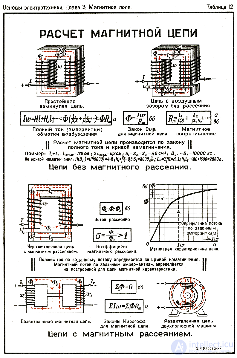
Calculation of a branched magnetic circuit
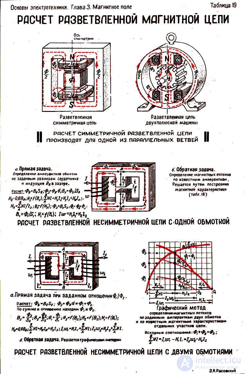
Answer:  .
.
Answer: 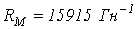 .
.
Answer:  .
.
 and cross section
  , if
, if  .
.


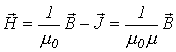 ,
,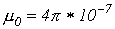
 H/m- the magnetic constant
 of the magnetic core

 where
where  -current in the winding,
 -number of winding turns
 , where
  and
and  are the boundary points of the section of the magnetic circuit for which
  is determined
 ,obtained through a series of repeated, sufficiently slow changes of the magnetic field strength within a chosen range
 (see curves 1 in Fig. 1).
 and is usually close to the basic magnetization curve





 equals the product of the magnetic flux and the reluctance
  of that section





Comments