
Lecture
An electrical filter is a two-port network placed between a power source and a load, serving to pass currents of some frequencies with little (unimpeded) attenuation while blocking (or passing with high attenuation) currents of other frequencies.
A filter in electronics is a device for extracting the desired components of the spectrum of an electrical signal and/or suppressing undesired ones.
An electrical filter is a device or system used to filter electrical signals or electromagnetic waves in order to extract the required information from noise, interference, or other unwanted signals.
Depending on the type of filter, it can be designed to suppress or attenuate certain frequencies of a signal, or to pass only frequencies within a certain range. Electrical filters are widely used in various fields, including radio electronics, telecommunications, audio and video engineering, medical equipment, the automotive industry, etc.
The most common type is the bandpass filter — a filter that passes components lying within a certain frequency band.
A bandpass filter is a linear system and can be represented as a sequence consisting of a high-pass filter and a low-pass filter.
Ideal bandpass filters are characterized by two parameters
 ;
; .
.In turn, a practical implementation of a bandpass filter is characterized by six parameters
 ;
; .
. ;
; ;
;as well as
 ;
; .
.An example of an implementation of such a filter can be a resonant circuit (a circuit of a series-connected resistor, capacitor and inductor).
There are several types of electrical filters, including
Each type of filter has its advantages and disadvantages, and the choice of a particular type depends on the requirements of the specific system or application.
The range of frequencies passed by a filter without attenuation (with low attenuation) is called the passband or transmission band; the range of frequencies passed with high attenuation is called the attenuation band or stopband. The quality of a filter is considered to be higher the more pronounced its filtering properties are, i.e. the more strongly the attenuation increases in the stopband.
As passive filters, two-port networks based on inductors and capacitors are usually used. It is also possible to use passive RC filters, used at high load resistances.
Filters are used both in radio engineering and communications technology, where currents of sufficiently high frequencies occur, and in power electronics and electrical engineering.
 ), and the capacitive susceptances of the capacitors are much greater than their active conductances (
  ).
).The filtering properties of two-port networks are caused by the resonant modes that arise in them – resonances of currents and voltages. Filters are usually assembled as a symmetrical T- or Pi-shaped circuit, i.e. with  or
or  (see Lecture No. 14). In this connection, when studying filters we will use the concepts of attenuation coefficient and phase coefficient introduced in the previous lecture.
The classification of filters according to the range of passed frequencies is given in Table 1.
Table 1. Classification of filters
|
Filter name |
Range of passed frequencies |
|
Low-frequency filter (low-pass filter) |
|
|
High-frequency filter (high-pass filter) |
|
|
Bandpass filter (band-pass filter) |
|
|
Notch filter (band-stop filter) |
 and and  , where , where  |
In accordance with the material presented in the previous lecture, if a filter is loaded with a resistance that equals the characteristic impedance at all frequencies, then the voltages and, correspondingly, the currents at its input and output are related by
.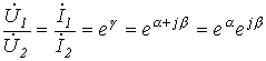 . . |
(1) |
In the ideal case, in the passband (transparency band)  , i.e. in accordance with (1)
  ,
,  and
and  . Consequently, the equality
  also holds, which indicates the absence of losses in an ideal filter, and therefore an ideal filter must be built from ideal inductors and capacitors. Outside the passband (in the stopband) in the ideal case
  , i.e.
  and
and  .
.
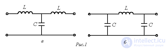
Consider the circuit of the simplest low-pass filter, shown in Fig. 1,a.
The relationship between the two-port network coefficients and the parameters of the elements of the T-shaped equivalent circuit is determined by the relations (see Lecture No. 14)

or specifically for the filter in Fig. 1,a
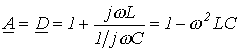 ; ; |
(2) |
 ; ; |
(3) |
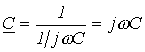 . . |
(4) |
From the two-port network equations written using hyperbolic functions (see Lecture No. 14), it follows that
 .
.
However, in accordance with (2)  is a real variable, and therefore,
 . . |
(5) |
Since in the passband the attenuation coefficient  , then on the basis of (5)
 .
.
Since the limits of variation of  are:
are:  , - the boundaries of the passband are determined by the inequality
 ,
,
which is satisfied by frequencies lying in the range
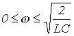 . . |
(6) |
For the characteristic impedance of the filter, on the basis of (3) and (4) we have
 . . |
(7) |
Analysis of relation (7) shows that as the frequency w increases within the limits determined by inequality (6), the characteristic impedance of the filter decreases to zero while remaining resistive. Since, when the filter is loaded with a resistance equal to the characteristic impedance, its input impedance will also equal  , then, due to the realness of
  , we can conclude that the filter operates in a resonance mode, as noted earlier. At frequencies greater than
  , as follows from (7), the characteristic impedance acquires an inductive character.
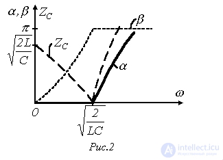
Fig. 2 shows the qualitative dependences  and
and  .
.
It should be noted that outside the passband  . Indeed, since coefficient A is real, the equality
 . . |
(8) |
must always hold. Since outside the transparency band  , relation (8) can only be satisfied when
  .
.
In the stopband, the attenuation coefficient  is determined from equation (5) at
  . What is significant here is the fact that
  gradually increases, i.e. in the stopband the filter is not ideal. A similar conclusion about the non-ideality of a real filter can be drawn for the transparency band as well, since it is practically impossible to ensure a matched operating mode of the filter throughout the entire passband, and therefore in the passband the attenuation coefficient
  will differ from zero.
Another variant of the simplest low-pass filter can be a two-port network built according to the circuit in Fig. 1,b.
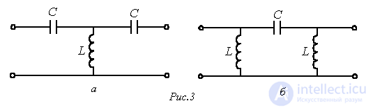
The circuit of the simplest high-pass filter is shown in Fig. 3,a.
For this filter the two-port network coefficients are determined by the expressions
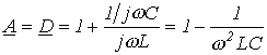 ; ; |
(9) |
 ; ; |
(10) |
 . . |
(11) |
As in the case considered above, A is a real variable. Therefore, on the basis of (9)
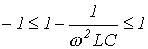 .
.
This inequality is satisfied by the following range of frequency variation
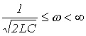 . . |
(12) |
The characteristic impedance of the filter
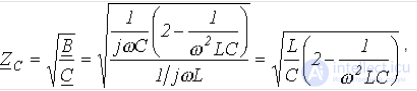 , , |
(13) |
varying from zero to  as the frequency increases, remains real. This corresponds, as already noted, to the filter, loaded with the characteristic impedance, operating in the resonant mode. Since such matching of the filter to the load throughout the entire passband is practically impossible, the filter actually operates with
  only within a limited frequency range.
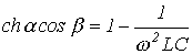
Outside the passband,  is determined from the equation
 |
(14) |
at  . The smooth variation of the attenuation coefficient in accordance with (14) shows that in the stopband the filter is not ideal.
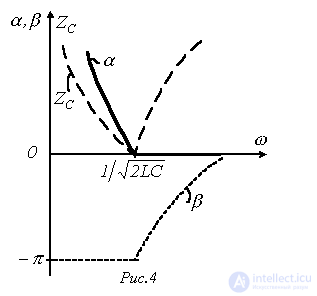
The qualitative shape of the dependences  and
and  for a low-pass filter is shown in Fig. 4.
It should be noted that another example of the simplest high-pass filter can be the Pi-shaped two-port network in Fig. 3,b.
A bandpass filter is formally obtained by connecting in series a low-pass filter with passband  and a high-pass filter with passband
  , where
  . The circuit of the simplest bandpass filter
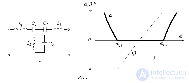
is shown in Fig. 5,a, and Fig. 5,b shows the qualitative dependences  for it.
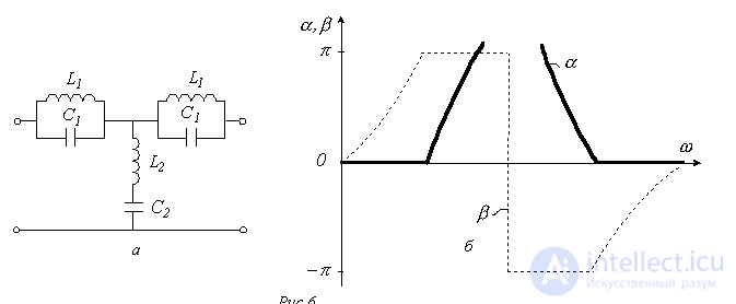
In a notch filter, the transparency band is divided into two parts by a stopband. The circuit of the simplest notch filter and the qualitative dependences  for it are shown in Fig.6.
In conclusion, it should be noted that to improve the characteristics of filters of all types it is advisable to build them as a ladder circuit, representing cascaded two-port networks. When a matched operating mode is ensured for all n sections of the circuit, the attenuation coefficient  of such a filter increases in accordance with the expression
  , which brings the filter closer to ideal.
Filters used in signal processing can be
Among the many recursive filters, the following filters are singled out separately (by the form of the transfer function):
By the order (degree of the equation) of the transfer function (see also the log-amplitude-frequency response), filters are distinguished as first-order, second-order and higher-order filters . The slope of the log-amplitude-frequency response of a 1st-order filter in the stopband is 20 dB per decade, of a 2nd-order filter — 40 dB per decade, and so on.
By which frequencies are passed (blocked) by the filter, filters are divided into
In the design of passive analog filters, lumped or distributed reactive elements such as inductors and capacitors are used. The impedance of reactive elements depends on the signal frequency, so by combining them it is possible to achieve amplification or attenuation of harmonics of the spectral components (which may not necessarily be harmonics) at the required frequencies. Another principle for building passive analog filters is the use of mechanical (acoustic) vibrations in a mechanical resonator of one design or another.
An RC circuit or an LR circuit can be used as the simplest low- and high-pass filters. However, they have a low slope of the frequency response in the stopband, which is insufficient in many cases: only 6 dB per octave (or 20 dB per decade) for an RC filter, which is a 1st-order filter, and 40 dB/decade for an LC filter, which is a 2nd-order filter. In passive filters, adding any reactive component to the filter circuit increases the filter order by 1.
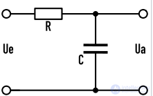 Passive 1st-order RC low-pass filter
The simplest 1st-order low-pass filter is shown in the figure and consists of a series-connected resistor  and capacitor
  , forming a voltage divider for the input signal. The complex transfer coefficient
  of such a divider is:

where  — is the time constant of the RC circuit.
The magnitude of the transfer coefficient of this circuit:
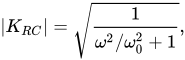
where 
At input frequency  the magnitude of the transfer coefficient is close to 1, at
  the magnitude of the transfer coefficient is close to 0, at frequency
  the magnitude of the transfer coefficient equals
 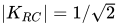 — a decrease relative to the unity transfer coefficient of approximately 3.01 dB; this frequency is called the cutoff frequency of the filter. In the stopband, at frequencies much higher than the cutoff frequency, the magnitude of the transfer coefficient decreases by 20 dB per decade of frequency change.
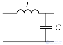
The figure shows an example of the simplest LC 2nd-order low-pass filter: when a harmonic signal of a certain frequency is fed to the filter input (on the right in the figure), the output voltage of the filter (right) in steady state is determined by the ratio of the reactances of the inductor (  ) and the capacitor (
  ).
).
The transfer coefficient of the LPF can be calculated by considering this filter as a voltage divider formed by reactances.
The complex (accounting for the phase shift between voltage and current) impedance of the inductor is  and the complex impedance of the capacitor is
  , where
  — is the imaginary unit,
  — is the angular frequency of the input harmonic signal, so for an unloaded LC filter the transfer coefficient will be expressed by the voltage-divider formula:
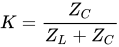 .
.
Substituting the expressions for the complex impedances into the formula, we obtain the frequency-dependent transfer coefficient:
 .
.
As can be seen, the transfer coefficient of an unloaded ideal LPF whose signal source is an ideal voltage generator with zero internal resistance grows without bound as the resonant frequency 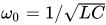 is approached, since the denominator of the expression tends to zero. As the frequency rises above resonance, it decreases. At very low frequencies the transfer coefficient of the LPF is close to unity, at very high frequencies — close to zero.
The dependence of the magnitude of the complex transfer coefficient of the filter on frequency is called the amplitude-frequency response (AFR), and the dependence of the phase on frequency — the phase-frequency response (PFR).
In real circuits, an active load is connected to the filter output, which lowers the Q factor of the filter and eliminates the sharp peak of the transfer coefficient near the resonant frequency  .
.
The quantity  is called the characteristic impedance of the filter
or wave impedance of the filter. If the LPF is loaded with an active resistance equal to the characteristic impedance, the transfer function becomes non-resonant, the transfer coefficient will be approximately constant for frequencies
is called the characteristic impedance of the filter
or wave impedance of the filter. If the LPF is loaded with an active resistance equal to the characteristic impedance, the transfer function becomes non-resonant, the transfer coefficient will be approximately constant for frequencies  , and will decrease as
  at frequencies above . At frequency the transfer coefficient of such an LPF decreases by 3 dB relative to its value at low frequency; this frequency is called the cutoff frequency of the filter. At frequencies much higher than the cutoff frequency, the transfer coefficient decreases by 40 dB per decade of frequency change.
An LC high-pass filter is built in a similar way. In the HPF circuit, the inductor and the capacitor swap places. For an unloaded HPF, the following expression for the transfer coefficient is obtained:
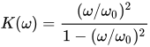 .
.
At very low frequencies the magnitude of the HPF transfer coefficient is close to zero. At very high frequencies — close to unity.
At ultra-high frequencies, lumped elements (capacitors and inductors) are practically not used, since as frequency increases their typical component values, and hence their dimensions, decrease so much that manufacturing them becomes impossible. Therefore, so-called transmission lines with distributed parameters are used, in which the inductance, capacitance, and active resistance are uniformly or non-uniformly distributed along the entire line. Thus, the elementary LPF discussed in the previous section consists of two lumped elements forming a resonator; in the case of distributed parameters, however, the filter consists of a single resonator element (for example, a section of microstrip line or a metal rod).
The designs of microwave filters are quite diverse, and the choice of a particular implementation depends on the requirements placed on the device (operating frequency values, Q factor, maximum attenuation in the stopband, location of spurious passbands).
Designing filters with distributed parameters is a fairly complex process consisting of two stages: obtaining the electrical parameters based on the device requirements, and obtaining the dimensional parameters from the electrical ones already obtained. Modern methods of microwave filter design are based on the theory of coupled resonators.
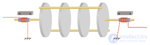
An electromechanical filter (EMF) contains a mechanical resonant system (resonator) of one design or another. Electromechanical transducers are located at the input and output of the filter, converting the electrical oscillations of the signal into mechanical vibrations of the filter's working element and back.
EMFs have become widespread in the intermediate-frequency stages of high-quality radio systems (including military, marine, amateur-radio and other systems). Their advantage is a significantly higher Q factor than that of equivalent LC filters, allowing high selectivity to be achieved, which is necessary for separating closely spaced radio signals in receivers.
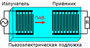
Active analog filters are built on the basis of amplifiers enclosed in a feedback loop (positive or negative). In active filters it is possible to avoid using inductors, which allows the physical size of devices to be reduced and simplifies and lowers the cost of their manufacture.
LC filters are used in power circuits to suppress interference and to smooth voltage ripple after a rectifier. In stages of radio-electronic equipment, tunable LC filters are often used; for example, the simplest LC tank circuit connected at the input of a medium-wave radio receiver provides tuning to a particular radio station.
Filters are used in audio equipment in multiband equalizers to correct the frequency response, to separate low-, mid- and high-frequency audio signals in multiband acoustic systems, in tape-recorder frequency-correction circuits, and elsewhere.
 ,
,  .
.
1. What is an electrical filter?
2. Which type of filter is used to suppress certain signal frequencies?
3. Which type of filter is used to pass only frequencies lying within a certain range?
4. Which parameter characterizes a filter's ability to suppress signals outside the given range?
5. Which type of filter has the lowest Q factor?
6. Which type of filter is used to amplify certain signal frequencies?
. Active and digital filters are not designed to amplify certain signal frequencies, but rather to filter or process the signal. An "amplification filter" is not a standard type of filter.
7. Which parameter characterizes the bandwidth of a filter's passband?
8. Which type of filter is used to reduce the noise level in an electrical signal?
9. Which parameter characterizes the ratio of the maximum signal to the noise level at the filter output?
10. Which type of filter has the highest Q factor?




Comments