
Lecture
The essence of the operator method is that a function  of the real variable t, called the original, is put into correspondence with a function
  of the complex variable
  , called the transform (image). As a result, derivatives and integrals of originals are replaced by algebraic functions of the corresponding transforms (differentiation is replaced by multiplication by the operator p, and integration – by division by it), which in turn allows the transition from a system of integro-differential equations to a system of algebraic equations for the transforms of the sought variables. Solving these equations gives the transforms, and then, by the inverse transition, the originals. The most important practical point here is that only the independent initial conditions need to be determined, which substantially simplifies the calculation of transients in high-order circuits compared with the classical method.
In the general case, the procedure for calculating transients by the operator method is as follows:
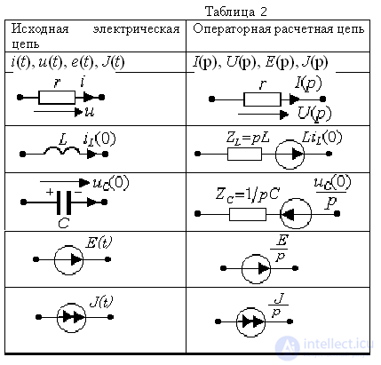
1) An operator equivalent circuit is constructed for the circuit that results after commutation, following the rule given in Table 1. Positive directions for the branch currents are chosen.
2) The pre-commutation state of the circuit is determined (the currents in the inductors and the voltages on the capacitors before commutation are found).
3) By any calculation method (using Kirchhoff's equations, the mesh-current method, the node-potential method, etc.), the operator transform of the sought quantity is determined.
4) Based on the transform obtained, the original of the sought function is found.
The operator method for calculating transients is based on the use of the linear integral Laplace transform, which makes it possible to reduce any integral and differential time relations to algebraic expressions, obtaining a system of algebraic equations that depend on the complex variable p
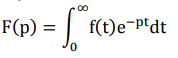
f(t) – the original, F(p) – the transform, ≓ - the symbol of correspondence between the original and the transform under the Laplace transform. Each function of time f(t) corresponds to a unique function of the variable p: ( ) ≓ ( ), and conversely, each function of the variable p corresponds to only one function of time: ( ) ≓ ( ). The transforms of the most frequently used functions are given in Table 1.
The transform  of a given function
  is determined in accordance with the direct Laplace transform:
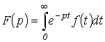 . . |
(1) |
In shorthand notation, the correspondence between the transform and the original is denoted as:
 or
or 
It should be noted that if the original  increases as t grows, then for the integral (1) to converge, a faster decay of the modulus
  is required. The functions encountered in practice when calculating transients satisfy this condition.
As an example, Table 1 gives the transforms of some characteristic functions frequently encountered in the analysis of non-stationary regimes.
Table 1. Transforms of typical functions
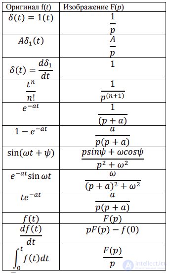
Original  |
Transform  |
| A |  |
 |
 |
 |
 |
 |
 |
 |
 |
 |
 |
Some properties of transforms
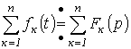 .
.
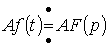 .
.
Using these properties and the data of Table 1, it can be shown, for example, that
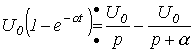 .
.
Transforms of the derivative and the integral
It is proved in the mathematics course that if  , then
 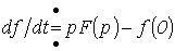 , where
  is the initial value of the function
  .
.
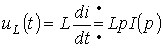
Thus, for the voltage across an inductive element, we can write
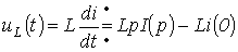
or, under zero initial conditions,
 .
.
Hence the operator impedance of the inductor
 .
.
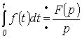
Similarly for the integral: if  , then
  .
.
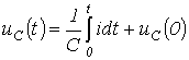
Taking non-zero initial conditions into account, for the voltage across the capacitor we can write:
 .
.
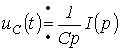
Then
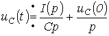
or, under zero initial conditions,
 ,
,
from which the operator impedance of the capacitor
 .
.
Suppose we have some branch  (see Fig. 1), separated out of some
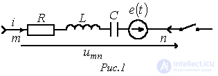
complex circuit. Closing the switch in the external circuit causes a transient, during which the initial conditions for the branch current and the capacitor voltage are, in the general case, non-zero.
For the instantaneous values of the variables, we can write:
 .
.
Then, on the basis of the relations given above, we obtain:
 .
.
Hence
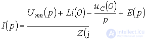 , , |
(2) |
where 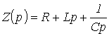 is the operator impedance of the section of the circuit under consideration.
It should be noted that the operator impedance  corresponds to the complex impedance
  of the branch in a sinusoidal-current circuit when the operator p is replaced by
  .
.
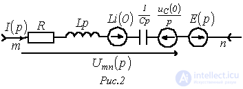
Equation (2) is the mathematical statement of Ohm's law, in operator form, for a section of a circuit with an EMF source. In accordance with it, for the branch in Fig. 1, an operator equivalent circuit can be drawn, shown in Fig. 2.
Kirchhoff's first law: the algebraic sum of the current transforms meeting at a node is zero
 .
.
Kirchhoff's second law: the algebraic sum of the EMF transforms acting in a loop equals the algebraic sum of the voltage transforms across the passive elements of that loop
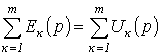 .
.
When writing equations according to Kirchhoff's second law, one must remember to take non-zero initial conditions into account (if present). With this taken into account, the last relation can be rewritten in expanded form as
 .
.
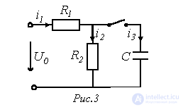
As an example, let us write the expression for the current transforms in the circuit of Fig. 3 for two cases: 1 -  ; 2 -
; 2 -  .
.
In the first case, according to Ohm's law, 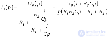 .
.
Then

and

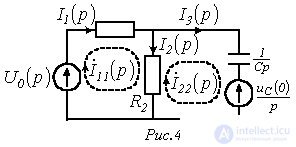
In the second case, i.e. for  , an operator equivalent circuit must be constructed for the circuit in Fig. 3, which is shown in Fig. 4. The current transforms in it can be found by any method for calculating linear circuits, for example, by the mesh-current method:
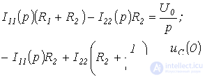
from which  ;
;  and
and  .
.
There are three ways of going from a transform to the original. The transition from the transform of the sought quantity to the original can be carried out in the following ways:
1. By means of the inverse Laplace transform The transition from the transform to the original is performed using the so-called Riemann–Mellin integral, which is the formula for the inverse Laplace transform:
, 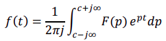
which represents the solution of the integral equation (1) and is written in shorthand as:
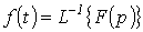 .
.
In practice, this method is rarely used.
Theorems that make it possible to represent the transform as a sum of simpler terms, thereby simplifying the transition from the transform to the original, are of great importance here.
2. Using correspondence tables between originals and transforms
The specialized literature contains a fairly large number of correspondence formulas covering practically all electrical-engineering problems. According to this method, the transform of the sought quantity must be brought to a form matching a tabulated one, after which the expression for the original is read off from the table. There are reference books containing several hundred transforms and their corresponding originals. One need only reduce the transform to the tabulated form. When using ready-made tables, one should find out which transform they were compiled with – Laplace or Carson. If the transform is given in the Carson form, it should be divided by p to obtain the Laplace transform.
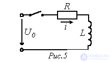
For example, for the current transform in the circuit of Fig. 5, we can write
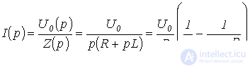 .
.
Then, according to the data of Table 1,
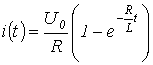 ,
,
which corresponds to the known result.
3. Using the expansion formula
The expansion theorem is used when the transform is found in the form of a rational fraction:

Where F1(p) and F2(p) – are polynomials in p
Let the transform  of the sought variable be given by the ratio of two polynomials
 ,
,
where  .
.
This expression can be represented as a sum of partial fractions
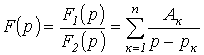 , , |
(3) |
where  is the k-th root of the equation
  .
.
To determine the coefficients  , multiply the left- and right-hand sides of relation (3) by (
  ):
):
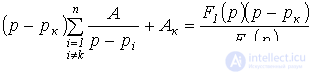 .
.
At 
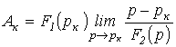 .
.
Treating the resulting indeterminate form of type  by L'Hopital's rule, we write
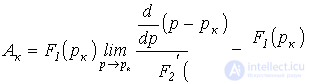 .
.
Thus,
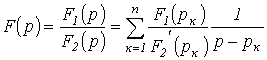 .
.
Since the ratio  is a constant coefficient, taking into account that
  , we finally obtain
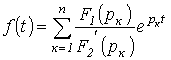 . . |
(4) |
Relation (4) is the expansion formula. If one of the roots of the equation  equals zero, i.e.
 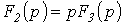 , then equation (4) reduces to the form
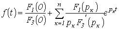 .
.
In closing this section, we note that to find the initial  and final
  values of the original, the limiting relations
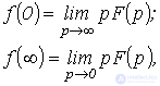
can be used, which can also serve to check the correctness of the transform obtained.
When working with transforms, one can use the properties of the Laplace transform, which make it possible to simplify the operator transform of the sought
function. It is obvious that the correspondence between the original and the transform is one-to-one, i.e. each function f(t) corresponds to one perfectly
definite function F(p) and vice versa. The most frequently used properties are given below.
Linearity property. When the original is multiplied by a constant, the transform is multiplied by the same constant:
af(t) ≓ aF(p).
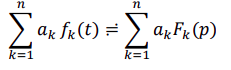
If the original is represented as a sum of functions, then the transform of this sum equals the sum of the transforms of these functions (the transform of a linear combination of
functions is a linear combination of transforms):
Differentiation theorem. Suppose some function f(t) has the transform F(p) , then the transform of the derivative of this function is

Computing the derivative under zero initial conditions (f(0) = 0) corresponds to multiplying the transform of the function by the factor p:

repeated differentiation under zero conditions:

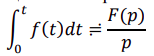
Integration theorem. The transform of some function f(t) is known. The transform of the function that is the integral of f(t) is determined by
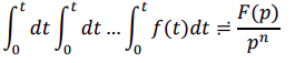
Repeated (n-fold) integration corresponds to the general expression:
Delay theorem. This theorem makes it possible to determine the transform of the function f(t - t1) , which differs from the function f(t) in that it is shifted
to the right along the time axis by t1 (Fig.1) :

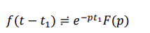
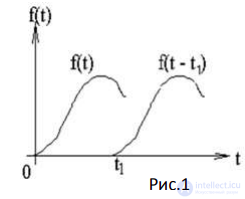
Thus, delaying a function by a time t1 corresponds to multiplying its transform by  .
.
Shift theorem. The shift theorem makes it possible to determine how the transform changes when the original is multiplied by the exponential
function e ±at, where a is a constant number.
Let the new function have the form
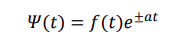
Its transform

Thus, multiplying a time function by an exponential factor leads to a «shift» in the transform domain of the independent
variable p by p±a
Theorem on the multiplication of transforms (convolution theorem – the Borel integral).
The theorem states the following: if
 , then

Thus, the product of the transforms of two functions corresponds to the convolution of their originals. The convolution theorem is widely used in
compiling tables of operator relations. If the transform of the sought function can be represented as a product of two (or more)
factors, then the original of the initial function can be computed from the originals of each factor.
Similarity theorem. This theorem makes it possible to determine the transform of a time function when the scale of its argument is changed. Suppose the transform of
the function f( t) ≓ F(p ). The transform of the function j(t) = f (at) , where a is some positive constant, will be
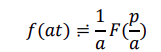
Multiplying the argument of the original by a positive constant a leads to dividing the argument of the transform and the transform itself by the same
number a.
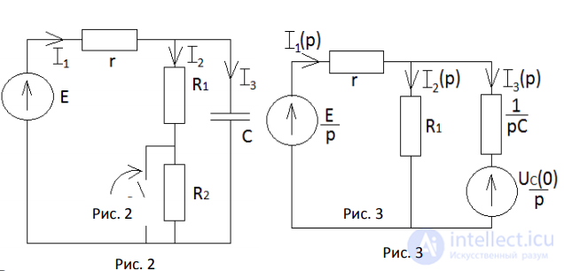
Solve the problem by the operator method. The circuit diagram, element parameters and EMF are as follows: E=100 V, r=10 Ω, R1=40 Ω, R2=50 Ω, C=1000 µF. Find the branch currents and the voltages on all circuit elements when the switch is closed: i1(t), i2(t), i3(t), UR1(t), UR2(t), UC(t), Ur(t).
Solution.
1. We construct the operator equivalent circuit for the circuit after commutation, using Table 1 (Fig.3):
2. We determine the pre-commutation state of the circuit.
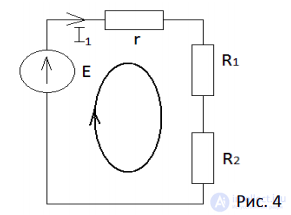
Here we need to determine the voltage across the capacitance UC(0), knowing that by the commutation law UC(0)=UC(0-). For this, we go back to Fig.2. Before
commutation, a constant current flows in the circuit that does not pass through the capacitance, so we replace it with a break in the circuit. This means the current
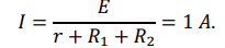
closes through the first loop. The circuit takes the form shown (Fig.4). The numerical value of the current can be found by writing, for this loop, the equation
by Kirchhoff's second law: 
terminals as R1 and R2 , that is, in parallel with these resistors, equals:

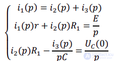
3. Let us determine the operator transforms of the sought quantities. The problem can be solved by any known method (using Kirchhoff's
equations, the mesh-current method, the node-potential method, etc.). We will use Kirchhoff's equations. This circuit has three branches and two
nodes, so one node equation and two loop equations must be written:
 (5)
(5)
Now let us express the current i2(p) from the second equation of the system in terms of the current i1(p) :
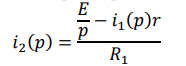 (6)
(6)
And then, substituting
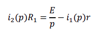
into the third equation of system (5), let us express the current i3(p) in terms of the current i1(p):
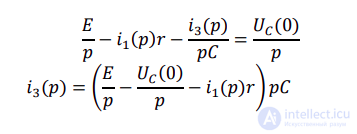 (7)
(7)
After this, expressions (6) and (7) can be substituted into the first equation, thus obtaining an equation for i1(p)

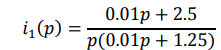
Substituting the known values of the EMF E, the value UC(0) found in step 2, the resistance values, and simplifying the expression, we obtain the operator transform
of the current i1:
 (8)
(8)
Now, using formulas (6) and (7), we can determine the operator transforms of the currents i2(p) and i3(p):
 (9)
(9)
 (10)
(10)
4. Let us now find the originals of the obtained quantities, using different methods.
- First, let us find the original of the current i1(t). Since the numerator and denominator of the expression obtained (8) are polynomials in p, and the fraction
is a proper rational fraction (the order of the numerator is less than the order of the denominator), we pass from the transform to the original by the expansion theorem.
- Let us write the numerator:
 . , the denominator
 let us find the derivative of the denominator:


Setting the denominator equal to zero, let us determine its roots:
p1=0; p2= -125
Substituting the roots, let us find the values of the numerator and of the derivative of the denominator:


Now the original of the current i1(t) can be obtained using the formula:
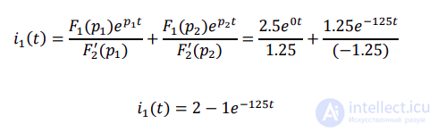
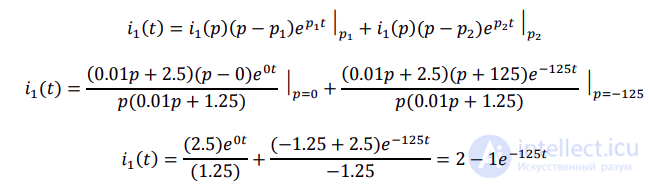
It is also interesting to obtain the original of the current i1(t) by the residue theorem; here too the denominator must be set equal to zero and its roots determined. The number of residues (terms) to be found will equal the number of roots:
- Let us now proceed to finding the original of the current i2(t).
- Here it is necessary to note that the expression consists of two terms, and to recall the linearity property: the transform
of a linear combination of functions is a linear combination of transforms. That is, we will look for the original of the first term, and then the original of the second. It is easy to see that the original of the first term is simply the constant – 2.5. The original of the second term will be found using the expansion theorem.
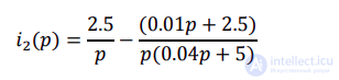
The transform of the current i2:
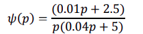
The second term:
The roots of the denominator are the same, since the transient process is unified throughout the circuit:  ,
,
1 . Let us write the numerator: 
, the denominator 
, let us find the derivative of the denominator: 
Substituting the roots, let us find the values of the numerator and of the derivative of the denominator:


Now we can obtain the original of the function ψ(t)

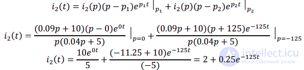
and then the original of the current i2(t) using the formula:

- Let us obtain the original of the current i2(t) by the residue theorem:
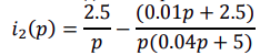
Let us bring both terms to a common denominator and simplify:

Let us find the current i2(t):
- The current i3(t) can be found in various ways: using the first equation from the system of Kirchhoff's equations, find the difference between the currents i1 and i2,
operating with the transforms and then passing to the original; or use expression (7), find the transform of this current and then pass to
the original in a convenient way; or find the difference of the originals of the currents i1 and i2 directly. The two latter approaches are the simplest:
- The transform of the current i3 from expression (7):

In simplified form:
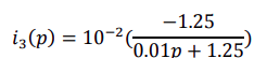
Here, in passing to the original, one must also recall the linearity property: when the original is multiplied by a constant, the transform
is multiplied by the same constant, and vice versa.
By the expansion theorem: 

By the residue theorem:

- Subtracting the originals directly:

It remains to determine the voltages across all the elements of this circuit: UC, UR1, UR2,

The voltage across resistor R2 dropped to 0 at the instant of commutation, and we take this change to be instantaneous, just like the commutation process itself.
The voltage across resistor R1 before commutation is 40 V (UR1= IR1), and after commutation it equals the voltage across the capacitance.
Using the active two-terminal network theorem, write the operator transform for the current through the inductor in the circuit of Fig. 6.
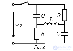
Answer: 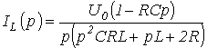 .
.
8. Using the limiting relations and the solution of the previous problem, find the initial and final values of the current in the branch with the inductive element.
Answer: 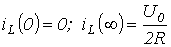 .
.

Comments