
Lecture
Classification of test and diagnostic equipment. Oscilloscopes, spectrum analyzers, AM/FM signal generators, generators
of LF, generators of HF, TV signal generators, analog microvoltmeters, digital multimeter, RLC meter, digital IC tester, semiconductor device tester,
At present, automatic monitoring and diagnostic systems solve a wide range of tasks. These primarily include:
It is natural to assume that all of the listed tasks should, if possible, be solved by the diagnostic system in real time.
An important characteristic of diagnostic systems is the diagnostic depth. This characteristic determines the level of diagnostics performed within the hierarchy of the technical system. Diagnostics can be carried out down to the level of individual devices making up the technical system, units, and components.
To date, a large number of types of technical diagnostic systems have been created, which, by identifying a number of significant distinguishing features, can be classified according to Fig. 11.2 [17].
By purpose, technical diagnostic systems can be divided into specialized and universal ones. Specialized systems are intended
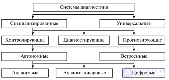
Fig. 11.2. Classification of technical diagnostic systems for diagnosing objects of a single type, and the list of monitored parameters and diagnostic algorithms is rigidly fixed and cannot be changed. Implementing such systems requires minimal equipment.
Universal diagnostic systems assume the possibility of evaluating the technical condition of various objects, monitoring a large number of parameters, and applying flexible algorithms.
Depending on the tasks solved by the diagnostic system, one can distinguish monitoring, diagnosing, and predicting systems. The purpose of monitoring systems is only to evaluate the operability of the object being diagnosed. This is the simplest type of task solved by a diagnostic system. For technical systems performing vitally important functions, this type of diagnostics may be preferable, since it can be implemented in real time, allowing timely measures to switch to backup systems. Fault-finding in this case is best carried out under stationary conditions.
Diagnosing systems make it possible to draw a conclusion not only about the operability of the diagnosed object, but also to indicate the failed device or component. The diagnostic depth depends on the degree of detail to which the diagnosed object is broken down into individual devices and components. For example, when a carburetor engine loses power, one can point to a fault in the fuel system, or one can pinpoint the failure by identifying a fault in the mixture-formation system in the carburetor.
A predictive diagnostic system makes it possible to assess the technical condition of the object under study at future points in time based on trends in the changes of monitored parameters.
By design type, diagnostic systems can be autonomous or built-in. Autonomous systems are implemented separately, outside the object being diagnosed. Their connection to the object is via special communication lines. For example, some rocket systems are monitored in flight mode by appropriate processing of telemetry data transmitted to the ground via radio signals. Built-in diagnostic systems are an integral part of the diagnosed object. All processing of diagnostic information in such systems is carried out on the object itself. Such systems are also called onboard systems.
And finally, by the form of signals and equipment used, diagnostic systems can be divided into analog, analog-digital, and digital. In cases where diagnostics is carried out using a small number of parameters that are continuous functions of time, and simple algorithms are used to process them, analog systems can be used. They are distinguished by high speed and reliability. At the same time, the accuracy of such systems is relatively low. If a computer is used in the diagnostic system to implement diagnostic algorithms, then its connection to sensors, whose output signals are usually continuous functions of time, is made via analog-to-digital converters. Such diagnostic systems are analog-digital. Purely digital diagnostic systems include either systems with a digital signal going from the sensor directly to the computer, or systems for diagnosing the computer itself.
The classification of diagnostic systems considered here is not exhaustive. Depending on the task at hand, it can be further deepened and expanded.
To build a diagnostic system, it is necessary to [17]:
Oscilloscope (Latin oscillo — to swing + Greek γραφω — to write) — an instrument designed for studying (observing, recording, measuring) the amplitude and time parameters of an electrical signal applied to its input, and visually displaying (visualizing) it directly on a screen, or recording it on photographic film.
Modern oscilloscopes make it possible to study signals in the gigahertz frequency range. For studying higher-frequency signals, electron-optical cameras can be used.
By operating logic and purpose, oscilloscopes can be divided into three groups:
Oscilloscopes with continuous sweep for recording a curve on photographic film (loop oscillograph).
By number of beams: single-beam, dual-beam, etc. The number of beams can reach 16 or more (an n-beam oscilloscope has n signal inputs and can simultaneously display n input signal traces on the screen).
Oscilloscopes with periodic sweep are divided into: universal (standard), high-speed, sampling, storage, and special; digital oscilloscopes can combine the ability to use various functions.
There are oscilloscopes (mostly portable) combined with other measuring instruments (e.g. a multimeter). Such devices are called scopemeters. In recent years, tablet oscilloscopes have appeared on the market, i.e. devices with fully touch-screen control on a color display.
An oscilloscope can also exist not only as a standalone instrument, but also as a computer add-on: in the form of an expansion card, or connected via some external port (most often USB).
An oscilloscope with a CRT-based display consists of the following main parts:
Auxiliary units are also included: brightness control unit, duration calibrator, amplitude calibrator.
Digital oscilloscopes most often use LCD displays.
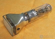
Oscilloscope cathode-ray tube
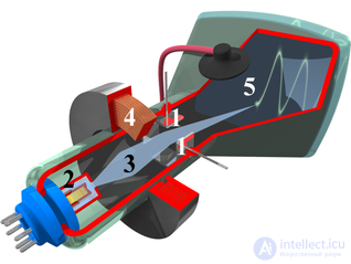
Diagram of an oscilloscope cathode-ray tube: 1 — deflection plates, 2 — electron gun, 3 — electron beam, 4 — focusing coils, 5 — screen
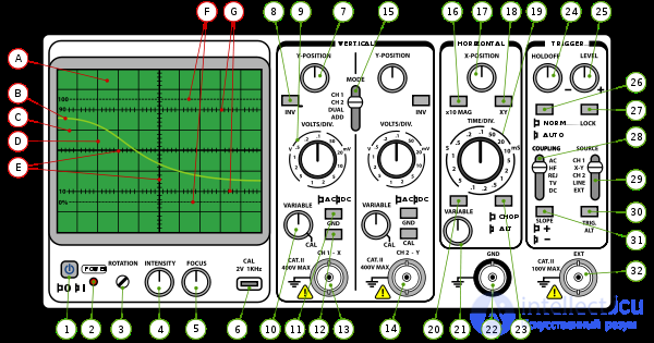
An oscilloscope has a screen A, on which the traces of input signals are displayed. In digital oscilloscopes, the image is output to a display (monochrome or color) as a ready-made picture; in analog oscilloscopes, the screen used is an oscilloscope cathode-ray tube with electrostatic deflection. The screen is usually marked with a coordinate grid.
Oscilloscopes are divided into single-channel and multi-channel (2, 4, 6, etc. input channels). Multi-channel oscilloscopes allow several signals to be observed simultaneously on the screen, their parameters measured, and compared with each other.
The input signal of each channel is applied to its own «Y» input and amplified by its own vertical deflection amplifier to the level required for the operation of the CRT's deflection system (tens of volts) or the analog-to-digital converter. The vertical deflection amplifier is always built as a DC amplifier (DCA), i.e. it has a lower operating frequency of 0 Hz. This makes it possible to measure the DC component of the signal, correctly display asymmetric signals relative to the zero line, and measure DC voltage. This mode of operation is called the DC-coupled mode.
However, if it is necessary to cut off the DC component (for example, if it is too large and drives the beam off the edge of the screen), the amplifier can be switched to AC-coupled mode (the input signal is applied to the DCA through a coupling capacitor).
Most oscilloscopes use two main sweep modes:
Some models also provide an additional mode:
Automatic sweep
With automatic sweep, the sweep generator operates in free-running mode, so even in the absence of a signal, once the sweep cycle ends — the cycle of the sawtooth sweep voltage generator — the next start occurs; this makes it possible to observe an image on the screen even in the absence of a signal, or when a constant voltage is applied to the vertical deflection input. In this mode, many oscilloscope models perform frequency locking of the sweep generator to the signal under study, with the sweep generator frequency being a whole number of times lower than the frequency of the signal under study.
Triggered sweep mode
In triggered sweep mode, on the contrary, when there is no signal or its level is insufficient (or the synchronization mode is set incorrectly), there is no sweep and the screen goes blank. The sweep starts when the signal reaches a certain level set by the operator, and the sweep start can be configured to trigger on either the rising or the falling edge of the signal. When studying pulse processes, even if they are non-periodic (for example, non-periodic, fairly rare shock excitation of an oscillatory circuit), the triggered mode ensures the visual stability of the image on the screen.
In the triggered mode, the sweep is often started not by the signal under study itself, but by some synchronous signal, usually leading the process under study, for example, a signal from a pulse generator that excites the process in the circuit under test. In this case, the triggering signal is fed to an auxiliary input of the oscilloscope — the sweep trigger input — the sync input.
Single trigger
In single-shot mode, the sweep generator is «armed» by an external action, for example, by pressing a button, and then waits for a trigger just as in triggered mode. After triggering, the sweep is performed only once; to trigger again, the sweep generator must be «armed» again. This mode is convenient for studying non-periodic processes, such as logic signals in digital circuits, so that subsequent sweep triggers on signal edges do not «clutter» the screen.
The disadvantage of this sweep mode is that the glowing spot traces across the screen only once. This makes observation difficult at fast sweep speeds, since the image brightness is low in this case. Photographing the screen is usually used in these cases. The need to photograph onto film was previously eliminated by using storage-type CRTs, and in modern digital oscilloscopes the process is stored digitally in the oscilloscope's digital memory (RAM).
To obtain a stationary image on the screen, each subsequent trajectory of the beam across the screen in the sweep cycles must trace the same curve. This is ensured by the sweep synchronization circuit, which triggers the sweep at the same level and edge of the signal under test.
Example. Suppose a sinusoidal signal is being studied and the synchronization circuit is configured to trigger the sweep on the rising edge of the sine wave, when its value equals zero. After triggering, the beam draws one or several sine wave cycles, depending on the configured sweep speed. After the sweep ends, the synchronization circuit does not re-trigger the sweep automatically, as in automatic mode, but waits for the next passage of the sine wave through zero on the rising edge. Obviously, the next pass of the beam across the screen will repeat the trajectory of the previous one. At sweep repetition rates above 20 Hz, due to the persistence of vision, a stationary picture will be seen.
If the sweep trigger is not synchronized with the observed signal, the image on the screen will appear «running» or even completely blurred. This happens because in this case, different sections of the observed signal are displayed on the same screen.
To obtain a stable image, all oscilloscopes contain a system called the synchronization circuit, which in foreign literature, not entirely correctly, is often called a trigger.
The purpose of the synchronization circuit is to delay the sweep trigger until some event occurs. In the example, the event was the sine wave passing through zero on the rising edge.
Therefore, the synchronization circuit has at least two settings available to the operator:
Correct adjustment of these controls ensures that the sweep is always triggered at the same point of the signal, so the signal image on the oscillogram appears stable and stationary.
Many oscilloscope models have another synchronization circuit control, a «STABILITY» fine-adjustment knob; changing its position changes the insensitivity time of the sweep generator to the triggering event (the «dead time» of the sweep generator). At one extreme position, the sweep generator switches to free-running mode, at the other extreme — to triggered mode, and at intermediate positions it changes the sweep trigger rate. Usually, oscilloscopes equipped with this control lack a «TRIGGERED/AUTOMATIC» sweep mode switch.
As mentioned, an additional sweep synchronization input is almost always provided, along with a «EXTERNAL/INTERNAL» sweep trigger switch; in the «EXTERNAL» position, the input of the sweep synchronization circuit is fed not by the signal under test itself, but by the voltage from the sync input.
There is often a switch for synchronization from the mains supply (50 Hz in European countries and Russia, 60 Hz in some other countries); with mains synchronization, the input of the synchronization circuit is fed with a voltage at the mains frequency. Such synchronization is convenient for observing signals at the mains frequency, or signals that are multiples of this frequency, for example, mains interference, when measuring the parameters of mains filters, rectifiers, etc.
Specialized oscilloscopes also have special synchronization modes, for example, a mode for triggering the sweep at the start of a line, numbered by the operator, in a television signal frame, which is convenient when measuring the parameters of a television path and its individual stages in television systems.
In other specialized oscilloscopes used for studying digital (for example, microprocessor-based) devices, the synchronization circuit is supplemented with a code comparator, and the sweep is triggered when a binary code (word) specified by the operator matches the code on the bus, for example, an address. This is convenient for locating the cause of malfunctions when writing/reading a particular memory cell and for other diagnostics.
One of the most important instruments in electronics. Used for applied, laboratory, and research purposes, for monitoring/studying and measuring the parameters of electrical signals — both directly and those obtained from the action of various devices/media on sensors that convert these actions into an electrical signal or radio waves.
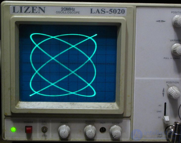
A Lissajous figure on the screen of a dual-channel oscilloscope
Oscilloscopes have a mode in which the horizontal deflection plates are fed not with a sawtooth sweep voltage, but with an arbitrary signal fed to a special input (the «X» input). If signals of close frequencies are applied to the «X» and «Y» inputs of the oscilloscope, Lissajous figures can be seen on the screen. This method is widely used to compare the frequencies of two signal sources and to fine-tune one source to the frequency of another.
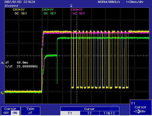
An example of displaying three processes under study on the screen of a modern oscilloscope, with two cursor markers. Time markers are displayed as vertical dashed lines; on the screen, white symbols on the left show the time between the markers — 40 ms — and the frequency corresponding to this time interval — 25 Hz.
Modern analog and digital oscilloscopes often have an auxiliary service system that conveniently measures certain parameters of the signal being studied by the oscilloscope. In such oscilloscopes, cursor images are additionally displayed on the screen showing the signal under test, in the form of horizontal or vertical lines, or in the form of mutually perpendicular straight lines.
The coordinates of the cursor lines by amplitude and time are displayed in decimal digital form, usually on the oscilloscope screen, or on additional digital indicators.
Using the cursor position controls, the operator can position a cursor on a point of interest on the signal image, while the cursor system continuously shows the coordinates of that point in digital form — the voltage level or the moment in time along the time axis and amplitude axis.
Many oscilloscopes have several sets of cursors, and the digital indicators can display the difference in values between a pair of vertical cursor markers and the time interval between a pair of horizontal cursor markers. In practically all types of such oscilloscopes, the value that is the reciprocal of the time interval between the cursor markers is automatically displayed in digital form on the indicators, which immediately gives the frequency of the periodic signal under test when the cursors are positioned along the time axis on adjacent signal edges.
Some oscilloscopes have an automatic cursor positioning mode on signal peaks, which in most cases is the goal of amplitude measurements. Thus, cursor measurements simplify signal parameter measurements for the operator, freeing them from the need to visually count the number of grid divisions on the oscilloscope screen scale and multiply the resulting data by the vertical and horizontal division values.
Some multichannel oscilloscopes have the ability to perform mathematical functions on the signals measured on different channels and display the resulting signal instead of or in addition to the measured original signals. The most common functions are addition, subtraction, multiplication, and division. This allows, for example, subtracting the synchronization signal fed to channel No. 2 from the signal under test on channel No. 1, thus freeing the signal under test from synchronization signals. Or, for example, it is possible to check the quality factor of an analog signal amplification unit by subtracting the input signal from the output signal. Some modern digital oscilloscopes have mathematical functions such as integration, differentiation, and square root extraction
In modern digital oscilloscopes, as well as in some specialized CRT-based oscilloscopes, there is a special synchronization mode - television. This mode allows displaying one or several specified television lines from a composite video signal. Unlike a regular oscilloscope, whose synchronization unit can stably show only the first line after the sync pulse, specialized oscilloscopes can observe any part of the television picture. Such oscilloscopes are usually used at television and cable studios and allow monitoring the technical parameters of transmitting and recording equipment.
Modern oscilloscopes do not require any calibration before use, but nevertheless most oscilloscopes have a built-in calibration device (Calibrator). The purpose of this device is to generate a reference signal with known and stable parameters. Usually such a signal has the form of rectangular pulses with an amplitude of 1 Volt, a frequency of 1 kHz, and a duty cycle of 50% (the parameters are usually indicated next to the calibrator signal output). At any time, the oscilloscope user can connect the instrument's measuring probe to the calibrator output and verify that the oscilloscope screen shows a signal with the specified parameters. If the signal differs from that specified on the calibrator, which is more typical for analog oscilloscopes, the user can use a trim screwdriver to adjust the input characteristics of the probe or the oscilloscope's amplifiers so that the signal matches the calibrator data. It should be noted that modern digital oscilloscopes do not have trim elements due to the use of digital signal processing, but they have automatic calibration adjustment, when a special utility is called through the oscilloscope menu that introduces correction coefficients into the oscilloscope's mathematical unit and thereby adjusts the oscilloscope for correct signal display.
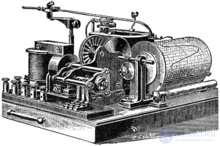
Hospitalier's ondograph
The electrical oscillatory process was initially recorded manually on paper. The first attempts to automate the recording were made by Jules Francois Joubert in 1880, who proposed a step-by-step semi-automatic method of signal registration. The development of Joubert's method resulted in the fully automatic Hospitalier ondograph. In 1885, the Russian physicist Robert Colley created an oscillometer, and in 1893 the French physicist Andre Blondel invented a magnetoelectric oscilloscope with a bifilar suspension.
The moving recording parts of the first oscilloscopes had high inertia and could not capture fast transient processes. This drawback was eliminated in 1897 by William Duddell, who created a light-beam oscillograph, using a small light mirror as the measuring element. The recording was made on a photosensitive plate. The pinnacle of the development of this method in the mid-20th century became multichannel strip-chart oscillographs.
Almost simultaneously with Duddell, Karl Ferdinand Braun used a picture tube of his own invention to display the signal. In 1899, the device was improved by Jonathan Zenneck, who added a horizontal sweep, which made it resemble modern oscilloscopes. In the 1930s, Braun's picture tube was replaced by Zworykin's picture tube, which made devices based on it more reliable.
At the end of the 20th century, analog devices were replaced by digital ones. Thanks to the development of electronics and the emergence of fast analog-to-digital converters, by the 1990s they had come to dominate among oscilloscopes.
Both digital and analog oscilloscopes have their advantages and disadvantages. The constant improvement of digital technologies makes it possible to create digital instruments that are more powerful and higher-performing compared to analog ones. At the same time, considering the simplest models of digital instruments, the price difference is constantly narrowing.
Listed below are the advantages and disadvantages of digital and analog oscilloscopes.
Advantages of analog oscilloscopes:
Disadvantages of analog oscilloscopes:
Advantages of digital oscilloscopes:
Disadvantages of digital oscilloscopes:
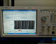
Logic analyzer
A logic analyzer is an electronic instrument that captures and displays multiple signals from a digital system or digital circuit. A logic analyzer can convert captured data into timing diagrams, protocol decoding, state machine traces, assembly language, or can correlate assembly with source-level software. Logic analyzers have advanced triggering capabilities and are useful when the user needs to see the timing relationships between many signals in a digital system.
A logic analyzer (Logic Analyzer) — is an electronic instrument that can record and display sequences of digital signals. It is used for testing and debugging digital electronic circuits, for example, when designing computer components and control electronic devices. Unlike oscilloscopes, logic analyzers have significantly more inputs (typically from 16 to several hundred), but are often only able to show two signal levels («0») and («1»), to which a «Z» state is sometimes added.
There are instruments that are a hybrid of logic analyzers and oscilloscopes, which allow the synchronous recording of digital and analog signals.
A logic analyzer can start recording on some trigger — a specific set of certain input lines. In some models, proprietary programs can be used to analyze the recordings obtained.
The largest manufacturers of logic analyzers: Agilent Technologies, Tektronix, LeCroy
Three different categories of logic analyzers are currently available on the market:
A logic analyzer can trigger on a complex sequence of digital events, and then capture a large amount of digital data from the system under test (SUT).
When logic analyzers first began to be used, it was common to attach several hundred «clips» to the digital system. Special connectors appeared later. The development of logic analyzer probes led to a common footprint supported by several vendors, which provides additional freedom for end users. Connectorless technology, introduced in April 2002 (defined by several vendor-specific trademarks: Compression Probing; Soft Touch; D-Max), became popular. These probes provide a durable, reliable mechanical and electrical connection between the probe and the printed circuit board with a load of less than 0.5-0.7 pF per signal.
Once the probes are connected, the user programs the analyzer with the names of each signal and can group several signals together to make manipulation easier. Then the capture mode is selected, either «timing» mode, where the input signals are sampled at regular intervals based on an internal or external clock source, or «state» mode, where one or more signals are designated as «clocks», and data is taken on the rising or falling edge of this clock, optionally using other signals to qualify this clock.
After selecting the mode, the trigger condition must be set. The trigger condition can range from simple (for example, triggering on the rising or falling edge of a single signal) to very complex (for example, configuring the analyzer to decode higher levels of the TCP/IP stack and trigger on a specific HTTP packet).
At this point, the user sets the analyzer to «run» mode, either running once or running repeatedly.
After the data is captured, it can be displayed in several ways: from simple (displaying signals or state lists) to complex (displaying decoded Ethernet protocol traffic). Some analyzers can also operate in «compare» mode, where they compare each captured data set with a previously recorded data set and stop the capture or visually notify the operator when this data set either matches or does not. This is useful for long-term empirical testing. Recent analyzers can even be configured to send a copy of the test data by email to an engineer upon a successful trigger.
Many digital designs, including microchips, are simulated to detect defects before the device is built. Simulation usually provides a logic analysis display. Often, complex discrete logic is verified by simulating input data and checking output data using boundary scan. Logic analyzers can reveal hardware defects that were not detected during simulation. These problems are usually too complex to model in simulation or too time-consuming to simulate, and often cross several clock domains.
Field-programmable gate arrays have become a common measurement point for logic analyzers, and are also used to debug logic circuits.
With the advent of digital computing and integrated circuits in the 1960s, new and complex problems began to arise that oscilloscopes had trouble handling. For the first time in the history of computing, it became necessary to view a large number of signals simultaneously. Early solutions attempted to combine the hardware of several oscilloscopes into a single package, but the clutter on the screen, the lack of well-defined data interpretation, and probing limitations made this solution exceptionally unsuitable for use.
The HP 5000A logic analyzer, introduced in the October issue of the Hewlett-Packard Journal, was probably the first commercially available instrument to be called a «Logic Analyzer». However, the HP 5000A was limited to two channels and presented information using two rows of 32 LEDs. The first truly parallel instrument was the twelve-channel HP 1601L, a plug-in module for the 180 series oscilloscope mainframes, which used the oscilloscope screen to display 16 rows of 12-bit words as 1s and 0s. It was introduced in January 1974 in the Hewlett-Packard Journal.
Mixed signal oscilloscopes combine the functionality of a digital storage oscilloscope with a logic analyzer. Some of them include the ability to view analog and digital signals simultaneously, as well as trigger on digital or analog signals and capture others. Some limitations of mixed signal oscilloscopes are that they do not collect data in state mode, have a limited number of channels, and do not provide the analytical depth and understanding of a logic analyzer.
Spectrum analyzer — a device for observing and measuring the relative energy distribution of electrical (electromagnetic) oscillations across a frequency band.
A spectrum analyzer makes it possible to determine the amplitude and frequency of the spectral components that make up the process being analyzed. Its most important characteristic is resolution: the smallest interval in frequency between two spectral lines that can still be distinguished by the spectrum analyzer. A spectrum analyzer can produce the true spectrum only when the analyzed oscillation
  is periodic, or exists only within the interval
  . When analyzing processes of finite duration, the spectrum analyzer does not give the true spectrum
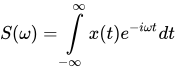 ,
,
but rather an estimate of it:
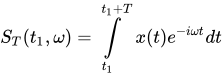 ,
,
which depends on the switch-on time  and the analysis time {\displaystyle T}. Since the spectrum of the oscillation can, in general, change over time, the estimate
  gives the so-called current spectrum.
LF analyzers come in parallel and sequential types (more often parallel) and are designed to work in frequency ranges from a few hertz to tens — hundreds of kilohertz. They are used in acoustics, for example, when studying noise characteristics, in the development and maintenance of audio equipment, and for other purposes. Analyzers used to monitor the quality of the power supply mains are otherwise called harmonic analyzers.
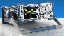
Spectrum analyzer FSL manufactured by Rohde & Schwarz
Most radio-frequency analyzers are wideband, allowing operation in a band from a few kilohertz to units — hundreds of gigahertz; as a rule, these are sequential-type analyzers. They are used to analyze the properties of radio signals and to study the characteristics of radio devices.
The most detailed information on the design principles of modern radio-frequency analyzers and their metrological characteristics can be found in the brochures "Spectrum Analysis Basics Application Note 150" by Agilent Technologies and "Fundamentals of Spectrum Analysis. Rauscher" by Rohde & Schwarz.
Sequential-type analyzers are the most common type of analyzer for studying radio signals; their operating principle consists of scanning the frequency band using a tunable local oscillator. The spectral components are sequentially converted to an intermediate frequency. Tuning the local oscillator frequency is equivalent to shifting the spectrum of the signal under study. A selective IF amplifier sequentially isolates the spectral components, and, thanks to the synchronous sweep of the oscilloscopic display, the responses of each spectral component are sequentially reproduced on its screen.
Parallel-type analyzers contain a set of identical narrowband filters (high-Q resonators), each tuned to a specific frequency (in the low-frequency measurement range, the filters may have the same relative frequency interval rather than the same absolute passband, for example, «third-octave filters»). When the signal under study acts on all filters simultaneously, each of them isolates the spectral component corresponding to its tuning. A parallel spectrum analyzer has the advantage of analysis speed over a sequential one, but is inferior to it in simplicity.
Digital analyzers can be built in two ways. In the first case, this is an ordinary sequential-type analyzer in which the measurement information, obtained by scanning the frequency band with a local oscillator, is digitized using an ADC and then processed by digital means. In the second case, a digital equivalent of the parallel type is implemented in the form of a DFT analyzer, which computes the spectrum using discrete Fourier transform (DFT) algorithms. Compared to sequential analyzers, digital parallel DFT analyzers have certain advantages: higher resolution and operating speed, and the ability to analyze pulsed and single-shot signals. They are capable of computing not only the amplitude spectrum but also the phase spectrum, and can simultaneously display signals in the time and frequency domains. Unfortunately, due to the limited capabilities of analog-to-digital converters (ADCs), parallel DFT analyzers operate only at relatively low frequencies.
Tektronix has created digital real-time spectrum analyzers. They make it possible to track rapid changes in the spectrum in real time, which are used in some types of modern communication systems. In addition to conventional spectra, these instruments allow spectrograms to be built, which represent a set of spectra displayed at different points in time. In addition, the instruments employ «digital phosphor» technology, which allows spectra to be stored for a certain time and their changes over time to be clearly tracked.
Rohde-Schwarz also manufactures real-time spectrum analyzers, in which a frequency mask triggering mode (selective triggering) is additionally implemented. In this mode, the spectrum analyzer triggers and takes measurements if the spectrum of the signal under study, within the analysis band of the parallel FFT analyzer based on an ADC, meets the specified conditions, for example, one of the spectral components at a given frequency exceeds a set level. This mode is useful for observing signal spectra in wireless communications, when it is possible to isolate the carriers or pilot signals that need to be studied.
Optical spectrum analyzers are built on the basis of a diffraction grating, Michelson interferometers, Fabry-Perot interferometers, and other interference schemes. Nowadays, due to their high manufacturability, analyzers using a diffraction grating are the most widespread, and only when their resolution proves insufficient are more expensive interferometric spectrum measurement methods used.
Optical spectrum analysis, in connection with the development of telecommunications technology, is becoming one of the most important types of measurement in modern fiber-optic communication systems. The need for this type of measurement is primarily related to monitoring the spectrum of optical radiation sources, as well as determining the degree of influence of spectral components on the parameters of fiber-optic components and data transmission over fiber-optic communication lines. At the same time, one of the significant factors currently limiting the bandwidth of high-speed communication lines is the chromatic dispersion of the optical fiber, which is determined by the width of the radiation source spectrum and manifests itself as an increase in the duration of the transmitted pulse as it propagates through the optical fiber, which also requires optical spectrum analysis. In addition, the introduction of fiber-optic amplifiers into communication lines, in particular EDFA (erbium-doped fiber amplifiers), and the development of WDM (wavelength division multiplexing) technology in telecommunications, make optical spectrum analysis during the installation and operation of fiber-optic transmission lines (FOTL) the most relevant type of measurement.
No sooner had mixed-signal oscilloscopes entered our everyday use than, in the past year of 2011, Tektronix Corporation — the world leader in oscilloscopy — announced the release of a new revolutionary product: a mixed-signal oscilloscope with a built-in, fully functional radio-frequency spectrum analyzer. The new series of instruments was designated MDO4000 and complements the well-proven DPO/MSO4000 closed-architecture oscilloscopes from Tektronix. On December 14, 2011, at the Elektra European Electronics Industry Awards competition (UK), the new instrument became the winner in the «Best Product of the Year» category among test and measurement equipment. This award was intended for the model deserving the title of the most interesting new product among test and measurement equipment for the past year. The article gives readers a detailed introduction to the capabilities of the new combined instruments.
The name of the MDO series comes from the words Multi-Domain Oscilloscope, that is, oscilloscopes operating in different signal-definition domains. There are now three of them (Fig. 1a):
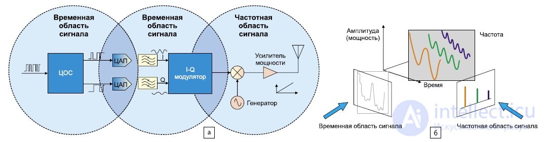
Fig. 1. Three domains for defining and measuring signals: a) block diagram of a modern wireless transmitter module; b) the time and frequency domains of a signal
Just about ten years ago, separate instruments were used in each of these domains — oscilloscopes, logic analyzers, and spectrum analyzers. All of these were complex, expensive, fairly large, and typically digital instruments. They considerably cluttered up the desks of engineers and scientists, and required substantial expense for purchase and maintenance. To use them in one's work, one had to additionally complete a special training course.
Work in each domain can be regarded as a measure or coordinate in measurements. Working in three domains lends measurements a three-dimensionality that, of course, should not be directly equated with purely geometric concepts. This three-dimensionality of signal representation by MDO-class oscilloscopes opens up new possibilities for obtaining a variety of information about signals with regard to the specific fields of their application. For example, signals from ordinary pulse devices are defined in the time analog domain, digital and pulse signals in the time digital domain, and signals from various radio-engineering and communication devices in the frequency domain. Now all of them can be studied with a single instrument from the MDO4000 series.
The MDO oscilloscope series includes four models (Table 1). The instruments are supplied to many countries, including Russia. A description is also available in Russian, running to 251 pages.
Table 1. Main parameters of the MDO4000 series oscilloscope — spectrum analyzers
| Model | Number of analog channels | Analog channel bandwidth, GHz | Analog channel sample rate, GS/s | Number of digital channels | Digital channel/MagniVu sample rate, GS/s | Operating frequency range |
| MDO4054-3 | 4 | 0.5 | 2.5 | 16 | 0.5/16.5 | 50 kHz...3 GHz |
| MDO4054-6 | 50 kHz...6 GHz | |||||
| MDO4104-3 | 1 | 5 | 50 kHz...3 GHz | |||
| MDO4104-6 | 50 kHz...6 GHz |
Note. MagniVu — the digital channel sample rate, increased through Tektronix's patented technology (when operating with enhanced time resolution — down to 60 ps).
The appearance of the instruments in the new series is shown in Fig. 2a. They resemble instruments in the DPO4000 and MSO4000 series (mixed-signal oscilloscopes).
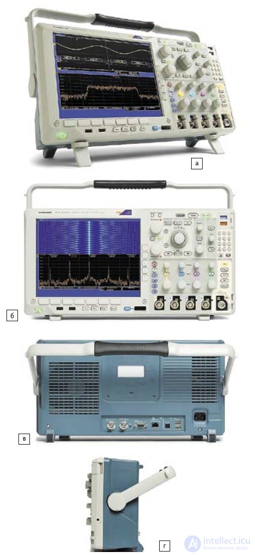
Fig. 2. MDO4000 oscilloscope: a) general view; b) front view; c) rear view; d) side view
The front view of the instruments is shown in Fig. 2b. The left half of the front panel is occupied by the instrument's screen. To the right and below it are the menu buttons. Below the bottom buttons are USB connectors, a group of buttons, and a connector for connecting digital and logic signal probes. The other half is occupied by the operating panel with the controls. A replaceable overlay with labels in languages other than English can be fitted onto it: for example, in Russian when instruments are supplied to Russia and the CIS countries. On the front panel there is a dual Wave Inspector knob for manual and automatic scrolling of waveforms. In the lower part of the panel are the controls for the four analog channels (their inputs are labeled with numbers from 1 to 4) and an additional radio-frequency RF input for the spectrum analyzer.
The rear view of the instrument is shown in Fig. 2c. In the center of the rear panel is a socket for attaching a security cable. Below (from left to right) are: an AUX Out connector, a reference oscillator output connector (10 MHz), an external display output connector, a connector for connecting to a local area network, universal serial bus (USB) connectors, and a connector for connecting the power cable.
The side view of the instrument is shown in Fig. 2d. There is nothing unusual here, except perhaps worth noting the «ground» socket for an antistatic wrist strap.
Fig. 3 shows a functional diagram of the simplified analog section of the instrument. Like the DPO/MSO4000 oscilloscope, it contains four analog inputs for signals examined by the oscilloscope section of the instrument. Below them is the new radio-frequency spectrum analyzer channel.
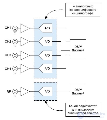
Fig. 3. Simplified analog section of the MDO4000 oscilloscope
The oscilloscope is supplied with a 16-channel digital probe and four analog passive probes. Active, differential, current, high-voltage, and other probes can be purchased separately. Fig. 4 shows the oscilloscope with probes connected to it. And Fig. 5 shows it with the RF channel probe connected. All channels can be connected simultaneously.
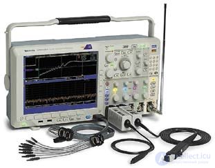
Fig. 4. MDO4000 oscilloscope with digital and ordinary analog signal probes
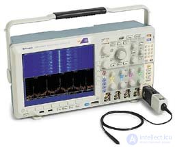
Fig. 5. MDO4000 oscilloscope with the spectrum analyzer's RF probe
A typical view of the oscilloscope screen is shown in Fig. 6. The screen consists of two parts. The upper part displays ordinary waveforms and logic diagrams, while the lower part displays the spectrum and spectrograms.
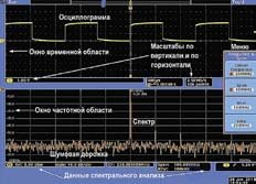
Fig. 6. Typical view of the MDO4000 oscilloscope screen
When operating in oscilloscope mode, the instrument has capabilities similar to those described for the DPO/MSO4000 oscilloscopes. It is worth recalling that these are the best of Tektronix's closed-architecture oscilloscopes. Thanks to a special memory, the instrument has a persistence property — digital phosphor. This makes it possible to observe waveforms of signals with rare signal anomalies — glitches (Fig. 7). Here, the rarer the glitches recur, the less brightly their waveforms are displayed. Nevertheless, being a digital storage oscilloscope, the instrument captures even single glitches. Fig. 7 shows that, if desired, the waveform can be expanded to fill the entire screen.
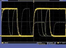
Fig. 7. Waveform of a pulse with glitches, illustrating the operation of digital phosphor
The oscilloscope section of the instrument makes it possible to observe waveforms of signals with strong time instability — jitter. An example of observing fast transitions with strong time jitter is given in Fig. 8. The upper part of the screen shows the construction of micro-histograms for evaluating the statistical parameters of jitter. The lower part of the screen shows a table of jitter parameters. A table of the results of automatic measurements performed by the oscilloscope is also displayed. Reference and calculated waveforms can be displayed if needed.
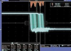
Fig. 8. Waveform of voltage transitions with strong jitter and its monitoring (above) using micro-histograms
In the upper right corner of the front panel there are two bays for plug-in oscilloscope software modules. They are supplied and purchased separately. There are modules for jitter analysis, power device and power supply research, testing of parallel and serial buses of various types, high-definition television devices, and others.
The presence of a radio-frequency spectrum analyzer within the MDO4000 series oscilloscopes is the main feature of these instruments. Here it is worth noting that software-based spectrum construction functions for waveforms are now present even in simple digital oscilloscopes. In some, in particular the DPO/MSO4000, they are implemented very well. They are especially good in the low-frequency range (signals with audio-range frequencies and the industrial AC mains), which is inaccessible to many radio-frequency spectrum analyzers. So what are the advantages of the MDO4000?
The main advantage is that the MDO4000 contains a channel of a fully-fledged spectrum analyzer with a separate radio-frequency RF input. A comparison of the MSO4000 spectrum analyzer with the software spectrum analyzer of an ordinary digital storage oscilloscope (DSO) and a mass-market spectrum analyzer is given in Table 2. It should immediately be noted that high-quality spectrum analyzers with a bandwidth of tens or even hundreds of GHz [4, 5] are of course far superior in their characteristics to the MDO4000, and comparing them makes no sense at all. It's like comparing a «Zhiguli» with a huge open-pit mining dump truck.
Table 2. Comparison of the MDO4000 with a DSO and a mass-market spectrum analyzer by main parameters
| Parameter | MDO4000 | DSO | Spectrum analyzer — standalone instrument |
| Frequency range | 50 kHz...6 GHz | DC…3.5 GHz | 100 kHz…3 GHz |
| Noise, dBc | –60...–50 | –45 | –60…–40 |
| Residual noise, dBm | –90...–80 | –70 | –90...–70 |
| DANL, dBm/Hz | –152 | –125 | –123 |
From this data it can be concluded that the spectrum analyzer of the MDO4000 oscilloscope occupies an intermediate position between ordinary DSOs and mass-market spectrum analyzers. The instruments have a uniquely wide spectrum capture bandwidth — more than 12 GHz! This allows analysis of most radio-frequency devices with signal frequencies up to 3 and even 6 GHz. However, their lower frequency boundary of the spectrum is fairly high — 50 kHz.
Since there is usually a time correlation between different areas of analysis, precise time interval measurements can be made to determine delay and wait times between events, evaluate command propagation time, and RF spectrum changes. For example, viewing the spectrum when a PLL VCO is powered on, or measuring transient characteristics during a step change in RF signal frequency, are now fairly simple tasks. Determining the source of irregular, hardware-dependent electromagnetic interference has never been so simple, thanks to the ability of the MDO4000 to provide a complete system study with time correlation in both domains, which is simply impossible to achieve with any other modern test and measurement equipment.
Externally, the difference between the new instruments and the previous DPO/MSO4000 series of oscilloscopes is manifested in the presence of a small spectrum analyzer panel located on the right side of the front panel (fig. 3). Above it are connectors for connecting software modules for jitter analysis, serial buses, power sources, etc. Fig. 9 shows the spectrum analyzer panel with a set of additional menus created by its buttons. The panel also has numeric buttons that are used to enter frequency values and other spectrum analyzer parameters.
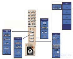
Fig. 9. MDO4000 spectrum analyzer panel and its associated menus
Joint display of waveforms and spectra is not always useful. But it often makes it possible to evaluate the operation of complex systems with various signals as a whole, tracking changes in particular signals over time. As an example, fig. 10 shows data on the operation of a sinusoidal signal synthesizer. The upper waveforms reflect the synthesizer's transient modes, while the spectrum of the signal below provides a frequency representation of the signal. It shows, in particular, that an amplitude-modulated signal is being formed with two sidebands adjacent to the carrier frequency spectral line.
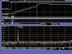
Fig. 10. Example of waveform and spectrum display
By moving the spectrum observation area, various components of it can be displayed (example in fig. 11). The spectrum analysis settings in DPO/MSO4000 oscilloscopes are not independent and are linked to the waveform settings. But the DPO4000 does not have this drawback: it has settings typical of dedicated spectrum analyzers. For example, the frequency range under study can be set by start and stop frequencies, or by center frequency and frequency span. There are other settings as well, familiar from dedicated spectrum analyzers.
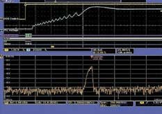
Fig. 11. Observing spectrum changes
A second example of this kind is given in fig. 12. Here another complex signal is being studied, and the spectrum (at the bottom of fig. 12) has a different appearance. The signal area for which the spectrum is built is marked by a characteristic bold line under the signal waveforms.
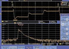
Fig. 12. Changing the spectral analysis time
An example of simultaneous display of a digital signal waveform and spectrum is shown in fig. 13. The spectrum is built for the signal applied to the RF input. The correspondence of the spectrum to a particular signal can be judged by the color of the signal and spectrum lines.
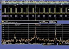
Fig. 13. Example of simultaneous observation of a digital signal and spectrum
If a detailed study of the spectrum is required, the entire window can be dedicated to its display so the spectrum can be viewed in maximum detail. An example of such a spectrum display is shown in fig. 14.
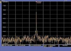
Fig. 14. Example of spectrum observation in an expanded window
In spectrometry practice, it is customary to mark various spectral lines or peaks with markers indicating their frequency and level. An example of such a marking for a single spectral line is given in fig. 14, and fig. 15 shows the use of markers to mark several spectral lines.
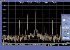
Fig. 15. Example of a spectrum with markers at the top of the spectrum window
The MDO4000 spectrum analyzer has a very effective means of averaging (Average) multiple spectra. This is especially useful for cleaning spectra of noise, impulse and high-frequency interference. The effectiveness of this tool can be seen in fig. 16. Here the averaged spectrum is shown by a white line. Averaging often makes it possible to clearly distinguish short, low-amplitude spectral peaks that may be masked by noise. However, it should not be forgotten that averaging increases the overall spectrum acquisition time.
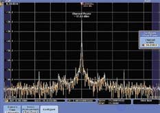
Fig. 16. Example of the spectrum averaging operation
Besides averaging, other operations are used when building spectra, such as capturing the spectrum maximum and minimum. The effect of these operations is demonstrated in fig. 17. The operations menu is shown on the right side of the window in fig. 17.
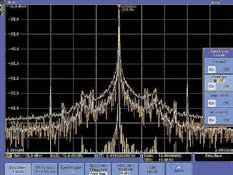
Fig. 17. Examples of spectrum operations and the operations menu
In the MDO4000 oscilloscope-spectrum analyzers, windowed fast Fourier transform (FFT) is used. In this case, the shape of the spectral peaks greatly depends on the type of window used. As an example, fig. 18 shows the Kaiser window, plotted on linear and logarithmic vertical scales. Such scales are also typical for spectrum plotting in general.
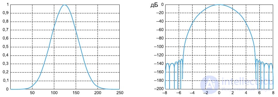
Fig. 18. Example of the Kaiser window on linear and logarithmic vertical scales
In the instruments under consideration, windows of various types can be set. An example of displaying RBW (resolution bandwidth) and window type (Window) when building a spectrum is shown in fig. 19. Note that RBW can be selected either manually (using the numeric keypad panel) or automatically.
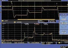
Fig. 19. Example of selecting RBW and window type when building a spectrum
Table 3 shows the parameters of possible window types used when performing spectral analysis with MDO4000 oscilloscope-spectrum analyzers.
Table 3. Types of spectral analysis windows
| Window | Window factor | Analysis time, μs |
| Kaiser (default) | 2.23 | 223 |
| Rectangular | 0.89 | 89 |
| Hamming | 1.3 | 130 |
| Hanning | 1.44 | 144 |
| Blackman-Harris | 1.9 | 190 |
| Flat-Top | 3.77 | 377 |
One of the powerful tools for spectrum research is the spectrogram. Spectrograms are built in the time-frequency plane, with the spectrum level represented by color. This uses a windowed fast Fourier transform. This type of spectral analysis is usually unavailable in simple spectrum analyzers. But it has been introduced in the DMO4000 (fig. 20).
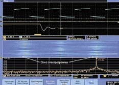
Fig. 20. Example of spectrogram window display
If necessary, the spectrogram window can be expanded and displayed together with a specified section of the spectrum. Such a case is shown in fig. 21.
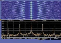
Fig. 21. Spectrogram window (top) and spectrum window (bottom)
One more important capability of the MDO4000 oscilloscope spectrum analyzer must be mentioned — viewing the spectra of individual channels in multichannel communication systems. Let us limit ourselves to the example shown in fig. 22. Here spectra are shown in three channels — the middle one with a high signal level, and the neighboring ones with a low signal level.
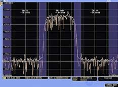
Fig. 22. Example of viewing the spectrum in a separate channel of a multichannel system
To improve the accuracy of spectral analysis in multichannel systems, averaging of multiple spectra is also used. The spectrum built with averaging is shown in fig. 22 by the white curve.
The DMO oscilloscope allows observation of various time dependencies, such as amplitude (callout 1 in fig. 23), frequency (callout 2 in fig. 23), and phase (callout 3 in fig. 23). Some of them are heavily contaminated with noise, which is particularly characteristic of the phase-versus-time dependence (fig. 23). Noise causes some dependencies to contain chaotic sections that it is desirable to remove. This is especially characteristic of the phase-versus-frequency dependencies. To highlight the desired dependencies and remove unwanted ones, an operation is provided for selecting the desired section of the dependencies and suppressing noise outside this section (fig. 24).
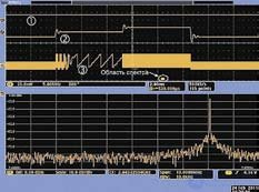
Fig. 23. Observation of various time dependencies and the spectrum of the signal at the RF input
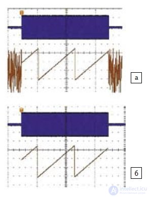
Fig. 24. Example of selecting a section of the phase-versus-time dependence and suppressing noise outside the selected section: a) noise suppression off; b) noise suppression on
The MDO4000 series oscilloscopes from Tektronix are the world's first combined instruments, uniting the functions of conventional digital storage oscilloscopes, digital and logic signal analyzers, and RF spectrum analyzers. The novelty of the development is evidenced by the filing of 26 patents, which are currently under review. The new instruments have a wide range of applications; in particular, they make it possible to study complex systems with various types of signals correlated in time .

Comments