
Lecture
The most important reliability indicator is the absence of failures during operation of a technical system. Technical diagnostics, through early detection of defects and faults, makes it possible to eliminate such failures during maintenance, which increases the reliability and efficiency of operation, and also makes it possible to operate critical-purpose technical systems on a condition-based basis. Under condition-based operation, each unit is operated until it reaches a limiting condition, in accordance with the recommendations of the technical diagnostics system.
The main task of technical diagnostics is recognition of the condition of a technical system under conditions of limited information.
The general theory of pattern recognition should be considered the theoretical foundation for solving the main problem of technical diagnostics. Technical diagnostics studies recognition algorithms as applied to diagnostic problems, which can usually be treated as classification problems.
Recognition algorithms in technical diagnostics are partly based on diagnostic models, which establish the relationship between the states of a technical system and their representations in the space of diagnostic signals. Decision-making rules are an important part of the recognition problem. To make a well-founded decision, it is advisable to use methods from the theory of statistical decisions.
Solving problems of technical diagnostics is always associated with forecasting reliability for the nearest period of operation (until the next technical inspection). Here, decisions must be based on failure models studied in reliability theory.
The second important direction of technical diagnostics is the theory of testability. Testability is the property of a product to ensure a reliable assessment of its technical condition and early detection of faults and failures. Testability is created by the design of the product and the adopted technical diagnostics system.
The state of a system is described by a set (collection) of parameters (features) that define it.
Recognition of the state of a system is the assignment of the system's state to one of the possible classes (diagnoses). The number of diagnoses (classes, typical states, reference states) depends on the specifics of the problem and the objectives of the study.
Often it is required to choose between one of two diagnoses (differential diagnosis or dichotomy), for example, "serviceable state" and "faulty state." In other cases, it is necessary to characterize the faulty state in more detail. In most problems of technical diagnostics, the diagnoses (classes) are established in advance, and under these conditions the recognition problem is often called a classification problem.
The set of sequential actions in the recognition process is called a recognition algorithm. An essential part of the recognition process is the selection of parameters describing the state of the system. They must be sufficiently informative so that, for the chosen number of diagnoses, the separation (recognition) process can be carried out.
Mathematical formulation of the problem. In diagnostic problems, the state of a system is often described using a set of features
K = (k1, k2, …, kj, …, kν), (2.1)
where kj – is a feature having mj grades.
Each grade (interval) of feature kj is denoted kjs. The actually observed state corresponds to a specific realization of the feature, which is marked with the superscript *.
In the general case, each system instance corresponds to a certain realization of the set of features:
 (2.2)
(2.2)
In many recognition algorithms it is convenient to characterize the system by parameters xj, forming a ν-dimensional vector or point in ν-dimensional space:
 (2.3)
(2.3)
In most cases the parameters xj have a continuous distribution.
Using feature kj a discrete description is obtained, whereas parameter xj gives a continuous description. With a continuous description, a significantly larger volume of preliminary information is usually required, but the description obtained is more accurate. If, however, the statistical distribution laws of the parameter are known, the required volume of preliminary information is reduced.
There are no fundamental differences in describing a system using features or parameters, and both types of description will be used further on.
As noted, in problems of technical diagnostics the possible states of the system – diagnoses Di – are considered known.
There are two main approaches to the recognition problem: probabilistic and deterministic. The formulation of the problem for probabilistic recognition methods is as follows. There is a system that is in one of n random states Di. A set of features (parameters) is known, each of which characterizes the state of the system with a certain probability. It is required to construct a decision rule by means of which the presented (diagnosed) set of features would be assigned to one of the possible states (diagnoses). It is also desirable to estimate the reliability of the decision made and the degree of risk of an erroneous decision.
With deterministic recognition methods, it is convenient to formulate the problem in geometric terms. If the system is characterized by a ν-dimensional vector X, then any state of the system is a point in ν-dimensional parameter (feature) space. It is assumed that diagnosis Di corresponds to a certain region of the feature space under consideration. It is required to find a decision rule according to which the presented vector X * (the object being diagnosed) will be assigned to a particular diagnosis region. Thus, the problem reduces to dividing the feature space into diagnosis regions.
In the deterministic approach, diagnosis regions are usually considered "non-overlapping," i.e., the probability of one diagnosis (in whose region the point falls) is equal to one, and the probability of the others is equal to zero. Similarly, it is assumed that each feature either occurs for a given diagnosis or is absent.
The probabilistic and deterministic approaches have no fundamental differences. Probabilistic methods are more general, but they often also require a significantly larger volume of preliminary information. Deterministic approaches more concisely describe the essential aspects of the recognition process, depend less on redundant, low-value information, and better correspond to the logic of human thinking.
The main advantage of statistical recognition methods lies in the possibility of simultaneously accounting for features of different physical nature, since they are characterized by dimensionless quantities – the probabilities of their occurrence under various states of the system.
In most recognition methods, the natural assumption is made that images of objects of the same class (pattern) are closer to each other than images of different classes. Metric methods are based on a quantitative assessment of this closeness. A point in feature space is taken as the image of an object, and the distance between points is considered the measure of closeness.
Experimental data providing statistical dependencies describing the relationship between a violation in the design of an object and a measured parameter can only be obtained for mass-produced objects. In some cases, such dependencies cannot be obtained. Then one way of obtaining the necessary information is to use equations describing the processes in the elements of the object, including the process of fault development, i.e., mathematical models of the object. As a result of calculations using both the object equations and the fault equations, the relationship between the degree of fault development and the behavior of the measured parameters is established, i.e., the information needed to form algorithms for functional diagnostic systems (FDS).
Mathematical models (MM) of system elements. A mathematical model (MM) of a system element – is a set of differential and algebraic equations, empirical formulas, tables, and graphs describing the characteristics of the element (unit, assembly), i.e., the relationships between internal and external control and disturbance parameters:
F (x, y, u) = 0,(2.4)
where x – is the vector of object parameters; y – is the vector of control actions; u – is the vector of disturbance actions.
For functional diagnostics problems, MMs are used in modeling (numerical experiment) the development of a particular fault in order to identify diagnostic features and verify the effectiveness of diagnostic hardware. There are MMs of a normally functioning element and MMs into which data on the development of a particular fault are incorporated. The latter MMs define the relationships between changes in design parameters causing abnormal operation of the object and the measured parameters. These two types of MM can differ substantially, since the occurrence of a fault can change the structure of the object and also leads to the appearance of a new variable characterizing the degree of fault development.
By the method of formation, MMs can be divided into analytical, empirical, and semi-empirical.
By the form of the equations used, or more precisely, by the depth of process description, all MMs are divided into linear and nonlinear. In addition, depending on the nature of the source data and the methods of processing it when forming the MM, semi-empirical and empirical MMs are divided into deterministic and stochastic. The ratio between the characteristic dimensions of the object under study and the length of the waves propagating in the object makes it possible to determine the need to use MMs describing the object as a system with distributed or lumped parameters.
From the ratio between the characteristic time constant of the system and the time of fault development, the question is resolved of whether it is necessary to account for dynamic processes in the system or whether it is possible to limit oneself to a quasi-static approach, i.e., to use static MMs. Analytical models contain differential equations, boundary and initial conditions for them, and algebraic relationships obtained from general physical laws. The advantage of analytical MMs – is their generality, the ability to describe processes in a sufficiently wide range of objects. The significant drawbacks of these MMs – are the low accuracy of describing the properties of many objects due to the complexity of real processes and the absence of sufficiently accurate analytical relationships for them, as well as the labor-intensiveness of finding solutions describing more or less complex processes, even using modern computers.
Empirical (experimental) models have sufficient accuracy; however, obtaining functional relationships between the parameters of the process in the object and external disturbances or regulating parameters requires a large volume of experiments. The results of experiments cannot always be extended to similar objects. To obtain generalized experimental dependencies suitable for describing processes in a number of objects of the same type, it is necessary to use methods of similarity theory.
Mixed semi-empirical MMs (mathematical models) are the most widespread; their formation uses both general physical laws and experimental data, which allow many process details not accounted for by analytical MMs to be taken into consideration.
In the case of forming purely empirical and semi-empirical MMs, identification methods are used to select the most convenient form of the equations and determine their coefficients. All of the listed types of MMs find application in the construction of TSD (technical diagnostic systems).
In nonlinear equations written in form (2.4), the variables x, y, u and their derivatives appear as products, powers, transcendental functions, etc. Linear (linearized) equations have the form
A(s) x = φ (y, u),2.5)
where A(s) – is a square matrix whose coefficients are polynomials in s; s = d / d t – is the differentiation operator. For linear equations there are well-developed solution methods, and the superposition principle is applicable to them; for nonlinear equations no such general solution methods exist. For most objects, including TSD, changes in process parameters over a sufficiently wide range are described by nonlinear relationships.
Depending on the class of problem being solved, the same object can be described by either nonlinear or linear (linearized) equations, and if the conditions for using the results of the solution allow it, it is always worthwhile, at least as a first approximation, to solve the linear (linearized) equation.
When constructing an MM, the admissible degree of model simplification is determined by the operating conditions of the system.
Models of objects consisting of interconnected elements (units, devices) are formed in two stages: first, the MMs of the processes in the individual components, units, and nodes of the system are created, and then the MM of the entire system is developed with the participation of the individual MMs of the subsystems and the structure of the connections between them.
Mathematical models of systems. To analyze the state of a system, the MM of the entire system must be assembled from the MMs of the elements; however, the totality of all the MMs of the elements making up the system is not yet the MM of the system. To form a closed system of equations, the connection equations between the parameters of the elements included in the MM must be added to the equations of the elements. If a diagram of the system is drawn, all the elements turn out to be interconnected, since information, working medium, electric current, energy, etc. are exchanged between them. For the sections or points connecting the elements, conservation laws are observed. In this case, it is convenient to apply the circuit theory apparatus.
Fault models. A fault model is understood as an analytical or stochastic relationship linking a parameter characterizing the degree of development of a fault with time or with the parameters of the diagnosed object. The primary structural parameters of the diagnosed object are usually used as the parameter characterizing the fault, since changes in these parameters are the cause of the appearance of fault indicators – changes in the measured parameters.
As a rule, MMs of simple faults are used, which are associated with a deviation from the normal value of the structural parameter of only one unit of the diagnosed object. The case of a complex fault, when the structural parameters of a number of units deviate from their normal values simultaneously (or in some sequence), is very inconvenient both for modeling and for diagnostics, owing to the diversity of possible combinations of parameters by magnitude, mutual sequence, etc.
If faults that disrupt the structure of the modeled system are being modeled, then the possible faults must be foreseen in advance in the MM in the form of separate structural elements.
To reproduce the pattern of fault development using the MM of an object, it is first necessary to determine the characteristic time over which the fault develops. If this time is comparable to or less than the characteristic time constant of the object, then it is necessary to use an MM of the diagnosed object that takes dynamic effects into account, i.e., terms with time derivatives. For such faults, the law of change of the primary indicators (parameter deviations) is given as a function of time:
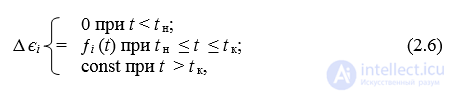
where Δ ei – is the deviation of the i-th primary structural parameter that is the cause of the development of this fault; t n – is the moment at which the primary parameter begins to deviate beyond the permissible limits; t k – is the moment at which measurement of the primary parameters ends; ƒi (t) – is the law of change over time.
Another variant of the ratio of characteristic times is possible, when the fault development time is much greater than the time constant of the object. In this case, a quasi-stationary MM of the object can be used, in which there are no terms with time derivatives.
Solving the problem of forecasting and ensuring technical service life involves establishing qualitative and quantitative relationships that determine the service life of equipment, and developing methods for assessing the influence of various factors on service life. Solving this problem opens up ways for scientifically substantiated assignment of service life, analysis and synthesis of equipment taking reliability factors into account, and for selecting design and technological solutions that ensure the assigned durability indicators.
Of particular interest is the problem of forecasting the individual service life of equipment based on the results of observations of its condition during operation. The limiting states of equipment are the result of the gradual accumulation of damage in parts, assemblies, and elements.
The concept of service life. Technical service life (hereinafter referred to as service life) – is a durability indicator characterizing the reserve of possible operating time of an object. Service life is the operating time of an object from the beginning or resumption of operation until the onset of a limiting state.
Any non-decreasing parameter characterizing the duration of operation of an object can be chosen as a measure of duration. Units for measuring service life are chosen individually for each industry and for each class of machines, units, and structures. From the point of view of theory and general methodology, the unit of time remains the best and most universal unit.
Calculating service life in units of time makes it possible to state forecasting problems in the most general form. Discrete time is sometimes used (for example, the number of on-off cycles or blocks). If the distribution of cycle or block durations is known, as well as the distribution of intervals between them, then converting to calendar time (or vice versa) presents no difficulty.
At the design stage, when the object has not yet been created, its calculation, including the estimation of service life, is performed on the basis of normative documents, which in turn are based (explicitly or implicitly) on statistical data on materials, actions, and operating conditions of similar objects. Thus, forecasting of service life must be based on probabilistic models. The assigned service life is set as a specific number corresponding to a certain probability with which the assigned service life must be realized in the designed object. The concept of gamma-percentile service life is usually used – the value of service life ensured with a given probability γ. The concepts of mean service life and mean operating life are also often used. At the design stage, these concepts mean the mathematical expectation of the service life and operating life, respectively.
Service life forecasting and reliability theory. Forecasting of service life – is an integral part of the theory of equipment reliability. Reliability is understood as the ability of a technical object to perform its specified functions over a specified period of time or specified operating time. The concept of reliability includes a number of properties of the object: failure-free operation, durability, maintainability, and storability. One of the central concepts of reliability theory is failure – an event consisting of a violation of the operable state of the object. In reliability theory, failure is treated as a random event, with the probability of failure-free operation over a specified period of time or within a specified operating time being taken as one of the main reliability indicators.
Service life and operating life, being durability indicators, also belong among the basic concepts of reliability theory. In the simplest situation, when an object is operated until the first failure, identified with the limiting states, the failure-free operation of the object simultaneously characterizes its durability as well. However, here we consider a more general case, when, after a run-in period, the failure rate is reduced to a minimum, and the system of scheduled preventive measures and maintenance guarantees the prevention of possible failures, or at least their rapid elimination without lengthy interruptions in operation and other undesirable consequences. Under these conditions, the main concepts become the limiting state, service life, and operating life.
The behavior of objects depends significantly on their interaction with the environment, as well as on the nature and intensity of the operating processes. In reliability theory, the properties of materials and actions are taken as random, so the behavior of the object is also random in nature. Normative requirements and technical operating conditions impose certain constraints on these parameters. The constraints can be formulated as the condition that a certain random vector, which depends on time and characterizes the quality of the object, lies within a given region. Failures and limiting states correspond to excursions of the random vector outside the region of admissible states. Thus, the main task of reliability theory – estimating the probability of failure-free operation over a given period of time – is reduced to the problem of outliers (level crossings) of random processes.
Intelligent systems based on artificial neural networks (ANNs) make it possible to successfully solve problems of pattern recognition, forecasting, optimization, associative memory, and control.
Like a biological neural system, an ANN is a computing system with a huge number of simple processors operating in parallel with numerous connections. ANN models reproduce, to some extent, the "organizational" principles characteristic of the human brain.
By analogy with the biological neuron, the artificial neuron also has synapses, a neuron cell, and an axon. The axon is the output connection of the neuron, through which the signal is transmitted to the synapses of the following neurons. Each synapse is characterized by the magnitude of the synaptic connection, or its weight wi, which in physical sense is equivalent to electrical conductivity. In the neuron cell, all inputs are summed, which determines the current state of the neuron.
The current state of the neuron is determined as a weighted sum of its inputs:

The output of the neuron is a function of its state:

The nonlinear function f is called the activation function and can take various forms. One of the most common is the nonlinear saturating function, the so-called logistic function or sigmoid (i.e., a function of S-shaped form):

An ANN can be regarded as a directed graph with weighted connections, in which artificial neurons are the nodes. By the architecture of their connections, ANNs can be grouped into two classes: feedforward networks, in which the graphs have no loops, and recurrent networks, or networks with feedback connections.
Obviously, the functioning process of an ANN, i.e. the essence of the actions it is capable of performing, depends on the values of the synaptic connections; therefore, having set a particular ANN structure suited to a given task, the network designer must find the optimal values of all the weighting coefficients.
This stage is called ANN training, and the network's ability to solve the problems set before it during operation depends on how well it is performed. At the training stage, besides the quality of weight selection, the training time also plays an important role. As a rule, these two parameters are related by an inverse dependence and have to be chosen based on a trade-off.
The most widespread training algorithm is the backpropagation algorithm. The essence of the algorithm is the propagation of error signals from the ANN outputs to its inputs, in the direction opposite to the forward propagation of signals in normal operating mode.
According to the least squares method, the minimized target error function of the ANN is the quantity:

where yjp( N )– the actual output state of neuron j of output layer N of the neural network when the p-th pattern is applied to its inputs; djp – the ideal (desired) output state of this neuron.
Summation is carried out over all neurons of the output layer and over all patterns processed by the network. Minimization is carried out by the gradient descent method, which means adjusting the weighting coefficients as follows:

Here wij – the weighting coefficient of the synaptic connection linking the i-th neuron of layer n-1 with the j-th neuron of layer n, η – the learning rate coefficient, 0 < h <1.
Nowadays the ANN method is actively used to solve the following energy and electrical engineering tasks: load prediction; forecasting ambient temperature for the purpose of load forecasting; controlling electric power flows in networks; ensuring maximum power; voltage regulation; power system diagnostics for the purpose of fault detection; optimizing sensor placement for power system safety monitoring; power system safety monitoring; ensuring transformer protection; ensuring stability, dynamic state estimation, and diagnostics of generators; turbogenerator control; generator network control; control of high-power switching systems; modeling of an induction motor; diagnostics and monitoring of transformer heating.
Let us consider the main possible directions for the application of NNs.
1. Application of NNs for parametric diagnostics of EMS components. It is based on comparing the mathematical model of a specific EMS component (motor, transformer, cable line, switching equipment) with the model of a defect-free component, i.e. checking whether the state parameters belong to the permissible ranges of their scatter. A parameter falling outside these ranges should indicate the presence of a fault in the corresponding node of the EMS component (fig.1).
2. Application of NNs for forecasting EMS parameters. An NN, based on a developed specific methodology, makes it possible to build the dependence of one parameter on another in the form of a polynomial. That is, it can help find hidden dependencies of one quantity on another, which cannot be determined by direct measurement methods. Thus, in an induction motor, by installing special sensors it is possible to measure, for example, the temperature of its individual parts in the stator. But measuring the temperature in individual parts of the rotor (magnetic core, winding, etc.) is difficult.
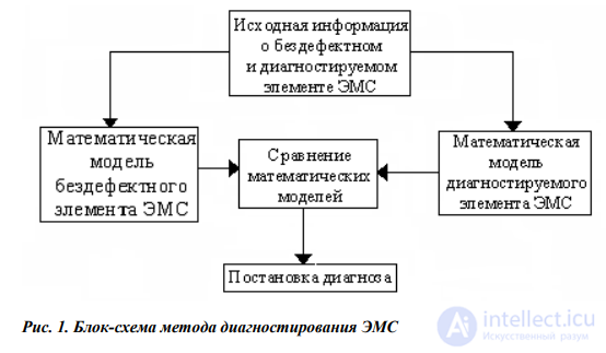
Using a thermal model of the motor developed for it, an NN will help
determine the temperature in given parts of the rotor for known
temperature values in the stator elements. Instead of temperature
any other parameter can be used.
3. Application of NNs for pattern recognition. Fault diagnostics
by many criteria coincides with the pattern recognition problem, therefore, using an NN, it is possible to achieve higher
results in detecting faults in electrical equipment that is part of an EMS compared to other diagnostic systems.
The state of any EMS component is characterized by a large
number of state parameters (features), whose values
can be obtained using standard measuring equipment, or
by carrying out additional tests on operating or
disconnected electrical equipment.
NNs make it possible to classify the state of electrical equipment, i.e. to assign its state to one of the classes
of states (sound, or faulty with a defect of a certain
type), determined from the given type of tests or measurements.
In diagnostic systems, experimental data on the features 
of each of the n recognizable operating modes can be determined both by direct measurements and on the basis of indirect measurements (fig. 2).
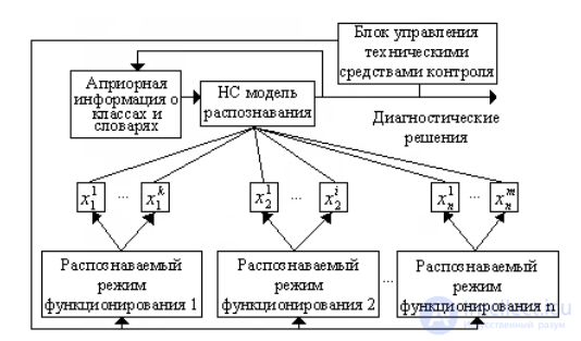
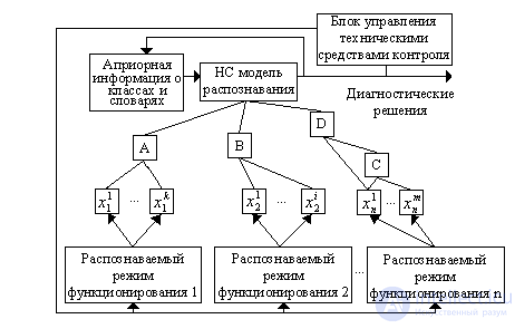
Fig. 2. Decision-making scheme in systems for recognizing the current technical state, with direct (left) and indirect (right) methods of obtaining information
Specialized local recognition systems are used for the latter.
Based on data from the n recognizable operating modes, primary features are determined. On the basis of primary features, second-level recognition devices A, B, C, D determine second-level features, and so on. The last group includes
features directly used in the process of recognizing unknown objects, i.e. features included in the working dictionary of features of the recognition system.
In NN theory, classification (clustering) is understood as the partitioning of a set of input signals into classes, given that
neither the number nor the features of the classes are known in advance. After
training, such a network is able to determine which class the input signal belongs to. The network can also signal that
the input signal does not belong to any of the identified classes — this is a sign of new data absent from the training
set. Thus, such a network can detect
new, previously unknown classes of signals. The correspondence between
the classes identified by the network and the classes existing in the
subject domain is established by a human. Clustering
is performed, for example, by Kohonen neural networks.
The number of inputs of a Kohonen network is the number of input parameters,
and the number of outputs is the number of faults. The number of outputs is less than
the number of input combinations. Thus, Kohonen networks recognize faults by classifying them depending on the set of
input parameters, which change from the nominal value to a
critical (maximum or minimum) value at which
failure of the object occurs.
Cluster analysis is a set of methods that make it possible to
classify multidimensional observations, each of which
is described by a set of characteristics (factors) X1, X2,..., Xm – in
this case this can be a set of signals from various sensors (state parameters of an EMS component). The goal of cluster
analysis is to form groups, classes of objects similar to one another,
which are usually called clusters. The word "cluster"
in translation from English means: a clump, bunch, group.
The following are used in the literature as related concepts: class, taxon, aggregation. In EMS systems, the classes in the simplest case can be two: "sound" and "faulty". As
a rule, the clear boundaries of each class are not specified, but their number
is known. When developing an EMS diagnostic system, cluster analysis based on a training set makes it possible to build a measure (distance) between the two main classes of objects
and determine the "centers" of each class in the space of characteristics X1, X2,..., Xm, i.e. to form the key rule for the diagnostic problem itself: for the presented object, distances are calculated to each of the classes ("sound" and "faulty"), and the object being classified is assigned to the class for which the distance turns out to be minimal.
In classification problems, the output element must produce
a strong signal if the given observation belongs to
the class of interest to us, and a weak one - in the opposite case.
In other words, this element must strive to model
a function equal to one in that region of the object space
where objects of the desired class are located, and equal to zero outside
this region.
The topology of such a network is characterized by the fact that the number
of neurons in the output layer, as a rule, equals the number of classes to be determined. In this case, a correspondence is established between
the output of the neural network and the class it represents. When the network is presented with a certain pattern, one of its outputs should show a sign that the pattern belongs to that class.
At the same time, the other outputs should show a sign that
the pattern does not belong to that class. If two or more outputs show a sign of belonging to a class, the network is considered
"unsure" of its answer.
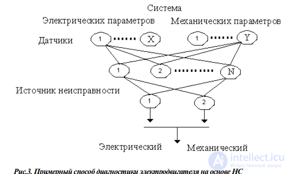
Let us give an example of an electric motor diagnostic system built on the basis of an NN (fig.3).
The motor state expert system has X sensors
monitoring the state of its electrical parameters (current,
voltage, etc.) and Y sensors monitoring the state of its
mechanical parameters (speed, vibration, temperature, etc.).
Each element of the input layer is assigned a possible value of the parameter. The output data was specified as a binary
vector, in which 1 corresponds to the presence of a fault, and 0
— its absence. Such a system will make it possible to determine the source
of the fault and its nature.
4. Application of neural network technologies for forecasting
the technical state of EMS. The forecasting ability of a neural network follows directly from its ability to generalize
and identify hidden dependencies between input and output data.
After training, the network is able to predict the future value
of a certain sequence based on several previous values or some factors existing at the current moment.
It should be noted that forecasting is possible only when
previous changes actually to some extent
predetermine future ones
If a set of values 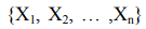 represents the values of some parameter changing over time,
then such a set is called a time series, with each value corresponding to the value of the parameter at a specific time  . The forecasting task in this case consists in
determining the value of the measured quantity X at time
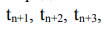 , that is, to carry out the forecasting it is necessary to
identify the pattern of this time series.
In neural networks, the forecasting problem is formalized
through the pattern recognition problem. Data on the predicted variable over a certain time interval form a pattern, the class
of which is determined by the value of the predicted variable at
some point in time beyond this interval, i.e.
the variable's value over the forecasting interval. The window
method involves using two windows Wi and Wo with fixed-
sizes n and m, respectively. These windows are able to move with a certain step along the time sequence of historical data, starting from the first element, and are designed to access the time series data, with the first window, Wi, receiving this data and passing it to the input of the neural network, and the second, Wo, to the output. The resulting pair at each step is used as an element of the training set (recognized pattern, or observation). Each subsequent vector is obtained by shifting the windows Wi and Wo one element to the right. The neural network, learning from these observations and adjusting its coefficients accordingly, attempts to extract these regularities and thereby form the required forecast function. As stated above, the result of a forecast using a NN is the class to which the variable belongs, rather than its specific value. Class formation should be carried out depending on the goals of the forecasting. The general approach is that the domain of the predicted variable is divided into classes in accordance with the required forecasting accuracy. Practical implementation of the listed properties of the NN will make it possible to create a fundamentally new system for automatic diagnosis and forecasting of the states of EMS subsystems
Review Questions
1 What is the primary task of technical diagnostics?
2 What is called a recognition algorithm?
3 How do the probabilistic and deterministic approaches to the problem of recognizing the technical condition of equipment differ?
4 How do analytical, empirical, and semi-empirical methods of forming mathematical models of objects and diagnostic systems differ?
5 Explain the patterns of behavior of the «life curve» of technical products.
6 What is the «damage measure» and how is it determined?
7 What is the «gamma distribution density»?
8 Explain the graph of the multi-stage model of the damage accumulation process.
9 What is the «technical service life» of equipment?
10 What is the difference between neural networks and conventional computing systems?
REFERENCES
1. Lyakhomsky A.V., Plashchansky L.A., Chebotaev N.I. et al. Electrification of Mining Production. In 2 volumes / Edited by L.A. Puchkov, G.G. Pivnyak, Moscow: MGGU Publishing House, 2007. – 1104 p.

Comments