
Lecture
For t > 3 geometric methods of verifying the Pareto-optimality conditions lose their clarity, and hence their effectiveness. The analogue of the preference angle becomes a region of three-dimensional space (y1, y2, y3), defined by the inequalities y1 > y*, y2 > y2, y3 > y3, except for the point itself (y*, y*2, y3). Geometrically, this region can be interpreted as the first octant of three-dimensional space (i.e., one of the eight parts into which space is divided by three coordinate planes), shifted by parallel translation from the origin to the point (y*, y, y3). The region is called the preference cone meaning not a cone in the usual sense (as a solid of revolution formed by the rotation of a straight ray about an axis), but a cone in the real vector space E, defined as a set K⊆E such that XK ⊆ K for any X > 0 . The complexity of spatial representations deprives the procedure of geometrically constructing the Pareto—Edgeworth set of the clarity inherent in the preference angle. Therefore, for t = 3 and for a larger number of criteria, the geometric interpretation usually loses its advantages. The image of the Pareto—Edgeworth set becomes a patch of a surface (or hypersurface for t > 3), the shape of which may turn out to be complex and inaccessible to visual representation.
Thus, the geometric verification of the Pareto-optimality conditions recedes into the background, and analytical and numerical methods become the priority.
Let us give a relatively simple and fairly general example, related to real financial and economic activity and illustrating the problems characteristic of such situations.
Example: consider a multi-criteria problem that arises in hedging (the transfer of price risk) — the use of options on future income in asset sale transactions.
Options are contracts that guarantee their buyer the right (but not the obligation) to sell (or buy) certain assets at an agreed price, thereby providing a means of protection against unfavorable price changes. At the same time, they leave open the possibility of profiting from favorable price changes. The payoff is not known in advance — it is a random variable that depends on the uncertainty of market conditions. Only a forecast is given, according to which the minimum income level V is ensured with probability 1 - α. The problem consists in optimizing over three criteria : obtaining the maximum level of the value V at the minimum probability of error and the minimum cost Q of purchase. The difficulties of the analysis are related to the fact that the payoff diagrams corresponding to options are more complex in form than the analogous diagrams for futures and forward contracts.
The Pareto—Edgeworth set corresponding to this multi-criteria problem is constructed using analytical estimates in the work of I. I. Gasanov and F. I. Ereshko for a certain class of constraints encountered in practice, and is shown in Fig. 9.5. Since, for the three criteria V, α, and Q, the Pareto—Edgeworth set O is three-dimensional, Fig. 9.5 shows the projection of 19 onto the plane of two criteria: the income level V and the α-quantile 5α of the distribution function E, the value of which at a given point equals α. The axis of the third criterion Q is directed perpendicular to the plane shown in Fig. 9.5, and depicting it would only make the illustration harder to perceive.
Note that the criterion 5α, which requires minimization, unlike all previous examples, has not been transformed in accordance with the remark at the beginning of the chapter, i.e., the direction of optimization here is not to the right and upward (as in previous cases), but to the left and upward. The Pareto—Edgeworth set O turns out to be a union of three subsets D1, D2 and D3, two of which (D2 and D3) project onto straight lines: D2 — onto the ordinate axis, and D3 — onto a line passing thr-
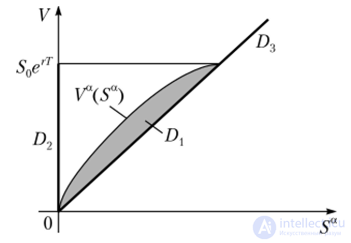
Fig. 9.5. Projection of the set of Pareto-optimal estimates in the option hedging problem through the origin. However, in three-dimensional space, D2, and D3 represent regions in the planes drawn through these lines and the axis Q. The set D1 is bounded in the plane of Fig. 9.5 by the curve E“(5“), where E“(5°) is defined as the root of the equation X(X0(Y)) = 5“ with respect to the variable V, where by '?(X) is denoted the expression
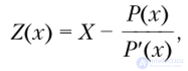
in which P(x) — is the given price of the asset.
Thus, the example of considering a multi-criteria problem confirms that, even when an analytical solution exists, the geometric interpretation, already in three-dimensional criteria space, lacks clarity and is not able to adequately provide a visual representation when projected onto a plane.
Note!
The conditions of Pareto-optimality are most easily verified geometrically using the preference angle in problems with two criteria. But in multi-criteria problems, geometric methods of verifying the conditions of Pareto-optimality are of little use and do not provide a simple and clear representation of the problem for decision-making. Moreover, projecting a multidimensional picture onto the plane of two criteria can lead to errors1.
Thus, the conditions of Pareto-optimality for t > 3 require other methods of analysis.

Comments