
Lecture
The relation (9.1) remains, even for m > 2, a relation of strict partial order , i.e., it possesses the properties of antireflexivity (y > y — not satisfied), antisymmetry ((y > y*) ∧ (y* > y) => (y = y*)) and transitivity ((y > y*) ∧ (y* > y**) => (y > y**)).
Note!
In contrast to R , in the space R"' there exist pairs of vector criteria y, y*, that either satisfy the relations y > y* or y* > y, or satisfy neither of these relations. Thus, the criterion space R™ — is a partially ordered group .
Let us illustrate the meaning of the criterion space as a partially ordered group geometrically for the case m = 2, i.e., for two criteria f1(x) and f2(x). For m = 3, i.e., in the criterion space R , the geometric interpretation becomes less illustrative. Let us give two examples corresponding to two frequently encountered (both in theory and in practice) types of the set of alternatives X: the discrete case and the region of possible options.
Example: a discrete set of alternatives. If the set of decisions X ⊂ R is discrete , i.e., all of its points are isolated , then it can be either finite (X = {x1 x2,xn}), or a countable set (X = {x1, x2,..., xn,...}). In practice, the situation of a finite set can arise if there are several (for example, n = 10) options of a product being purchased, of proposed projects, etc. The criteria in this case can, in particular, be y1 and y0 — price and quality (of the product, of the project).
To each alternative xk with number k let us assign the point Yk of the plane R2 with coordinates y1 = f1(xk) and y2 = f2(xk). Then the graphical representation, for n = 10, of the set of possible estimates Y = {y1, y2,..., y10} in the criterion space R2 is a collection of isolated points {Y1 Y2,..., Y10} (Fig. 9.1). Note that, in accordance with the assumption introduced at the outset, the criterion corresponding to price (say, y1), has been subjected to the transformation M - f1(x) so that the minimum price corresponds to the maximum value of y1. In this situation, the strict order relation introduced by formulas (9.1) can be interpreted in terms of the DM's preferences as follows. If two estimates y1 and yk satisfy the relation y. > yk, then the point Y- lies to the right of and above the point Yk, and then the DM can exclude the option yk as clearly less preferable compared to y..
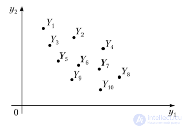
Fig. 9.1. A discrete set of possible estimates Y in a two-dimensional criterion space R2 and the image of the corresponding Pareto — Edgeworth set
From Fig. 9.1 it is evident that, although the set of possible estimates Y is not a linearly ordered set, i.e., all 10 alternatives cannot be arranged in a definite order, the partial ordering of the group makes it possible to single out from the set Y the points Y1 Y2, Y^ and Y8, located in Fig. 9.1 to the right of and above all the other options. In other words, when choosing the best decision, the DM can remove from consideration all the other alternatives and choose only among four: x1, x2, x4 and x8. Among themselves these options are incomparable according to formula (9.1). The values of the criteria y1 and y2 attain their maximum at different points: the criterion y1 attains its maximum at the point Y8, whereas the value y2 — at the point Y1, i.e., a simultaneous maximum on the set X is not achieved. The intermediate options Y2 and Y4 represent compromise solutions which may well correspond to the DM's preferences.
This narrowing of the set of alternatives X from the original 10 down to four, self-evident when looking at the illustration, ceases to be intuitive in the case of criterion spaces of higher dimensions m or for more complex sets of alternatives X. It is precisely the study, in the most general case, of this narrowing, called the Pareto — Edgeworth set, that constitutes the subject of this chapter.
The following example of a more complex set of alternatives X would naturally be called a continuous set (since continuity - is the generally accepted opposite of discreteness ), but formally in mathematics only linearly ordered sets are considered continuous . As we have seen, linear ordering is already absent for m = 2. Therefore let us call the set X a region, which, from the point of view of topology, is a connected subset of a topological space. A region is often taken to mean only an open set, but for decision theory it is more convenient to consider a closed region, i.e., the closure of the region, which also includes the boundary.
Example: a region as a set of alternatives. If the set of decisions X is connected, then between any «neighboring» alternatives, in terms of the values of the criteria, there can always be intermediate options. Then X must be an uncountable set. Such a situation arises, in particular, when choosing the optimal values of two control parameters (financial regulators, technical indicators, etc.) of some system, provided that the adjustment of these parameters can be carried out continuously within certain limits. A graphical representation of the set of possible estimates Y in the criterion space may look like a figure Y, shaded in Fig. 9.2.
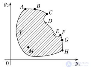
Fig. 9.2. The region of possible estimates Y in a two-dimensional criterion
space and the image of the corresponding Pareto — Edgeworth set
As in Fig. 9.1, the coordinates of each point in Fig. 9.2 (for example, the coordinates of the points A, B, C, I), E, B, C, Ya, M) represent the values of the criteria y1 and y2 for some alternative from the set X. But here, if the DM seeks to achieve the largest value of both criteria y{ and y2, i.e. their maximization is required, then the partial ordering of the group allows the DM to single out, from the set X, alternatives with images from the segments BC, OE and BC of the boundary of the shaded region Y, positioned, as in Fig. 9.1, to the right of and above all the other options. In other words, when choosing the best solution the DM can remove from consideration all the other alternatives with vector estimates from the shaded region Y and choose only points of the three indicated segments.
3
Note!
The ends of segments BC and GC remain among those of interest to the DM, while the ends of segment OE — do not, since they are dominated by points C and L respectively.
In this case, the narrowing of the set of alternatives, self-evident when looking at Fig. 9.2, all the more (compared to Fig. 9.1) ceases to be obvious in the case of criterion spaces of higher dimensions n or for more complex sets of alternatives X.
Note!
The two examples given show the importance of narrowing the set of possible estimates Y. If in the first example the choice from 4 alternatives becomes significantly simpler than the original choice from 10 options, then in the second — the number of alternatives is not simply reduced, but the original region Y with a finite area undergoes a qualitative transformation into a union of segments of a curved line having zero area.
The resulting narrowing of the set of alternatives X is called the Pareto — Edgeworth set (Francis Edgeworth1 (Francis Edgeworth, (1845—1926) — an English economist born in Ireland, who first, earlier than V. Pareto, introduced the concept of a Pareto-optimal solution for two criteria). It is precisely with the construction of this set that the analysis of any decision theory problem begins. Practical application of the indicated algorithm shows that often, as in the two examples given, narrowing X and constructing the Pareto — Edgeworth set restricts the set of remaining options so much that further choice is fairly simple and presents no difficulty for the DM.
Definition
Pareto — Edgeworth set, or set of Pareto-optimal solutions, is the name given to the set P/(X) of alternatives belonging to X x*, that are not dominated, i.e., for which there exists no dominating alternative x, satisfying the strict preference relation: x > x*.
From the definition it follows that to construct the Pareto - Edgeworth set, it is necessary to exclude from the set of solutions X all dominated alternatives. In other words, one must discard all such alternatives x* for which there exists at least one dominating alternative x > x*.
Note!
The practical significance of the Pareto — Edgeworth set is due to the fact that any solution x from the set of alternatives X, not belonging to PDX), is obviously unable to be optimal.
Indeed, by definition, solution x will be dominated with respect to some element x* of the Pareto — Edgeworth set, i.e., the DM will prefer x* to x.
Pareto-optimal solutions in the criterion space correspond to Pareto-optimal vectors (estimates).
Definition
Pareto-optimal vector (or Pareto-optimal vector estimate) is the name given to the vector /2(.x*), /m(x*)), corresponding to the Pareto-opti-
mal solution x*.
The examples given allow us to conclude that the main point of considering Pareto-optimal options and their vector estimates lies in the significant narrowing of the original sets X and Y, and moreover any of the remaining alternatives, by virtue of non-domination, may be recognized as optimal (best).
Note!
Pareto-optimal options, owing to the properties of their vector estimates, form a substantially narrower Pareto — Edgeworth set, compared with the original set X P^X). Thereby the DM's final choice of the best effective solution becomes much easier and simpler.
Along with the set of non-dominated alternatives, the set of non-dominated vector estimates is also considered.
Definition
The set of Pareto-optimal vector estimates, i.e., the image of the Pareto — Edgeworth set PXX) in the criterion space, is called the Pareto front[10] (sometimes the Pareto-front — from the English Pareto-frontier) or the Pareto — Edgeworth set in the criterion space.
From the properties of the algebraic structure, due to the linear ordering of the group, an important property of Pareto-optimal vector estimates follows.
Note!
Pareto-optimal vector estimates remain Pareto-optimal under any order-preserving linear transformations of the individual partial criteria.
In other words, such transformations of measurement scales as parallel translation (shift) along any axis of the criterion space, or a change of scale (i.e., of units of measurement) with a positive coefficient, do not change the property of Pareto-optimality.

Comments