
Lecture
The decision maker (DM) has stochastic («model-based» in terms of probabilistic models) information about the behavior of the environment. In this context, the following variants for describing the state of the environment are possible:
A decision-making problem under uncertainty – is a problem of choosing an optimal strategy whose outcome, besides the strategies of the operating side and a number of fixed factors (deterministic and stochastic), depends on uncertain factors that are beyond the control of the operating side and unknown to it at the moment of decision-making.
As a result of the influence of uncertain factors, each specific strategy (decision) corresponds not to a single outcome, but to a set of outcomes. The specific realization of the outcome for each decision is determined by the specific realization of the uncertain factors.
Let us consider the difference between fixed stochastic factors and uncertain factors. Both kinds of factors lead to a spread in the possible outcomes when the same decision is realized repeatedly. In this they resemble each other and differ from deterministic factors. The difference is that, with respect to fixed stochastic factors, the DM has the full completeness of statistical information – this information is sufficient for determining the probabilities of occurrence of the possible outcomes and for making a decision about choosing the optimal «on average» decision. With respect to uncertain factors, the DM does not have such information.
In what follows we shall consider the DMP under uncertainty without taking fixed stochastic factors into account.
With respect to the probabilities of realization of the various outcomes, two cases are possible (Fig. 4.1):
the probabilities of the possible outcomes have no physical meaning – then we are dealing with uncertain factors of a non-stochastic nature;
the probabilities of the possible outcomes have physical meaning, but are either unknown to the DM, or known with insufficient precision for decision-making – then we are dealing with uncertain factors of a stochastic nature.
Uncertain factors of a non-stochastic nature can be divided into two groups.
The first group consists of factors of strategic uncertainty – uncertain factors that arise from the participation of several operating sides in the operation. Each side is forced to make decisions under conditions in which the future actions of the other participants in the operation are unknown to it.
The second group consists of factors of conceptual uncertainty – uncertain factors that accompany the adoption of especially complex decisions having long-term or far-reaching consequences. In this case there may be vague, non-formalized goals (this, unfortunately, applies to a number of economic problems).
Decision-making problems under conditions of strategic uncertainty (or under conditions of a conflict situation) can be divided intosingle-level and multi-level.
In single-level decision-making problems, the participants are not bound by any form of subordination; they take part in a single operation and are interested in one or another of its outcomes.
Multi-level decision-making problems arise in complex control systems and have a hierarchical structure.
Single-level conflict DMPs can be antagonistic and non-antagonistic. In antagonistic ones, the interests of two sides pursuing directly opposite goals collide.
Uncertain factors of a stochastic nature include natural uncertainties.
Natural uncertainties – uncertain factors arising from insufficient knowledge of «nature».
In decision theory (DT), the term «nature» is understood to mean the entire set of circumstances under which a decision has to be made. These may be unknown characteristics of the processes associated with the course of the operation or the external conditions under which the operation is carried out.
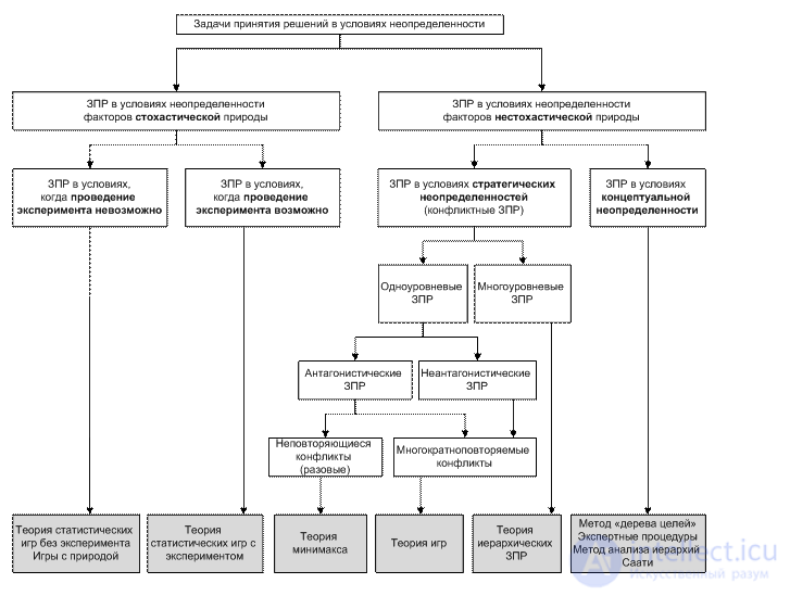
Fig. 4.1. Classification of DMPs under uncertainty
Figure 4.1 shows a «tree» of decision-making problems under uncertainty. The «leaves» of the tree explain which scientific fields, to one degree or another, remove uncertainty of the indicated kind. In more detail, in this textbook we shall focus on DMPs under uncertainty of factors of a stochastic nature. When conducting an experiment is possible, we suggest considering logical-probabilistic method (LPM); in cases where conducting an experiment is impossible, the apparatus of game theory against nature will help reduce the uncertainty.
Let us give two examples of decision-making problems for two different models of possible states of the environment S.
Example: a decision-making problem under conditions of certainty — a linear programming problem or a problem of optimal organization of production. The set of environment states consists of a single element.
Suppose that m types of raw materials are needed to produce a certain product. Using the equipment available at the enterprise, n production methods can be implemented, differing from each other in the composition of raw materials required to produce a unit of output.
Let us index the production methods by j = 1,2, ..., n, and the types of raw materials by index i = 1,2,..., m. Denote by a~ ∈ ℝ the amount of raw material of type i needed to obtain a unit of output by production method j. The stocks of raw materials are limited by the values b
A unit of output produced by method j brings a profit in the amount of cj conventional units (c.u.). It is required to organize production in order to obtain the maximum profit.
n The set of alternatives X for such a problem will consist of vectors x = (x1, x2,..., xn) ∈ ℝⁿ, called a production plan. In this case there are a number of constraints. First, the components of the vector must be non-negative numbers. Second, the quantities X representing the co-
j = 1
quantities of the i-th raw material, must not exceed the values ∈ ℝ, i = 1, 2,m. Thus, the set of admissible alternatives X will have the form

As the objective function, let us take the profit that can be brought by the production plan x = (x1, x2,..., xn) ∈ ℝ",
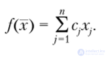
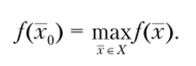
Thus, the solution of this DMP will be finding such a production plan (optimal plan) x0 = (x1, x2,..., xn) ∈ ℝ”, that maximizes profit under the given constraints, i.e.
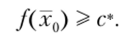
Note that this decision-making problem can also be considered under conditions where the sought plan (set of plans) must ensure that the DM's profit is not less than some predetermined (critical) value c* ∈ ℝ, i.e., the optimal production plan x0 = = (x,, x2,..., xn) ∈ ℝ” must satisfy the following inequality:
Example: a decision-making problem under conditions of probabilistic uncertainty — a problem of evaluating the efficiency of an investment portfolio. The set of environment states consists of an infinite, uncountable number of elements (continuum cardinality). A probability is explicitly defined on the set of states.
Suppose there is an investment portfolio containing two assets. The returns from investing a unit of capital in these assets are described by random variables ξ2, which, generally speaking, are not stochastically independent.
Suppose ξ1 has a uniform distribution on the interval [0, 12], i.e., the return of the first asset can be any value from 0 to 12%. Suppose ξ2 can take the values 2 or 10% with probabilities equal to 0.5, i.e., the second asset can, with equal probabilities, yield either 2% or 10%.
The investor wants to allocate a unit of the capital available to him between these assets in a way that is optimal in some sense.
In this formulation of the problem, the state of the environment is a two-dimensional real space S = ℝ2 with a given probabilistic structure (ℝ2, B2, P), where B2 — is the Borel σ-algebra, P — is the joint distribution of the vector ξ = (ξ1 ξ2). The set of alternatives X has the following form:

The set of outcomes of the decision R will be the set of values of the random variable Y representing the weighted average return of the portfolio 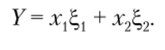
Thus, there arises a need to compare random returns. Let us define the evaluation function φ, for example, as the mathematical expectation of the random weighted average return

Then the more preferable decision will be the choice of such a vector x for which the mean value is greater

The set of best decisions can be constructed either as the set of vectors x for which the average return of the portfolio will be maximal. Obviously, in this numerical example, since the expression for the mathematical expectation E(Y) = x, • 6 + x2- 8.5 depends linearly on (x,, x2), one should take (x, = 0, x2 = 1).
An equally common criterion for choosing a decision is when the average return of the portfolio exceeds some predetermined threshold value M, for example, M = 7%:
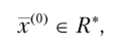
where R* — is the set of «good» decisions, if 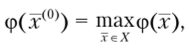 or
or
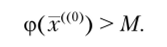
In this case, an acceptable managerial decision will be any pair (x,, x2), such that


Comments