
Lecture
Analytical methods, in the presence of nonlinear criteria and dependencies, also turn out to be too complicated and insufficiently effective; hence practice demonstrates the superiority of numerical procedures.
Note!
For three or more criteria, it is better to construct the Pareto — Edgeworth set using computer programs and algorithms.
In the case of a finite discrete set of alternatives X, consisting of n elements, the problem reduces to a pairwise comparison of alternatives. The total number of pairs equals  , in each pair one must carry out m comparisons
across all m criteria. Problems of this kind are implemented in many applied software packages, often as built-in functions. In practice, the numbers of alternatives n and criteria m are usually small, and in such cases the computation time on modern computers can be considered negligibly small.
However, for a set of alternatives X given in the form of a region, a fundamentally different situation arises. If there are no additional assumptions about the shape of the Pareto — Edgeworth set (for example, about its convexity), the computational complexity of the algorithm for finding it can be very high.
The simplest of such algorithms is the grid method , which is based on reducing the continuous case to a discrete one. For this purpose the original region X is covered by a fine grid with nodes at points X_i, i = 1,..., N, and then at all N nodes the vector estimates are calculated y_i = f(x_i). Here the number N rapidly increases as the dimensionality of the original region X increases, and can reach very large values. Among the estimates y_i, which make up a finite set of points in the criterion space, non-dominated vectors are selected by methods of pairwise comparison y*, forming a discrete approximation of the Pareto — Edgeworth set in the criterion space (or the Pareto front). The points of the original region corresponding to the estimates y*, points of the original region X (in other words, the preimages of the values y_i, i.e., y* = represent
a discrete approximation of the Pareto — Edgeworth set. For a continuous approximation (not only at the nodes but also between them) of the Pareto front, which represents a surface in an m-dimensional space, a polyhedron is used PN (determined by the number N of nodes), i.e., the collection of hyperplane segments passing through the grid nodes.
As practice shows, the grid method can require unacceptably high computational resources. Indeed, the following two types of situations are not uncommon.
For this reason, alternative methods are currently being intensively developed, based on «smarter» algorithms that save computational resources by taking into account the results of computations already performed in order to optimize subsequent procedures.
The class of «naive» methods, identified by Luke (S. Luke), is based on lexicographic tournament selection (lexicographic tournament selection ) and proceeds from the assumption that the individual criteria are ordered by importance, so that the most important is, for example, the criterion, the next in importance being the criterion f2(x) and so on. The idea of tournament selection itself is widely used in practical computations owing to its simplicity. Instead of a full set of comparisons of each of the N options with every other, a random sample of t alternatives is drawn — a tournament of t contenders is formed, within which all the alternatives are compared pairwise. Based on the results of the tournament, all dominated points are discarded, as well as all «worse» ones: for this a «fitness» function is defined (i.e., a fitness function similar to the objective function), by whose values the possibilities of two opposite outcomes are evaluated — either the alternative turns out to be dominated, or it enters the Pareto — Edgeworth set. Tournaments are repeated many times until practically the entire set of alternatives has been covered. The total number of comparison operations (i.e., the amount of computation as well) is significantly reduced, since a relatively small number  of comparisons makes it possible in each tournament to weed out a constant fraction of the alternatives. However, «naive» methods do not always work and are often not very effective. In practice it turns out to be difficult to choose either the «fitness» function or the tournament size t. For small values of t the probability of error is high — discarding points of the Pareto — Edgeworth set due to the random inclusion of «strong competitors» in the same tournament. For large t, comparable to N, the amount of computation decreases insufficiently fast because of the growing number of «redundant» comparisons.
In order to reduce the number of comparisons (and thereby the computational costs), adaptive algorithms have been developed, whose computational schemes adapt themselves to the situation, i.e., change their parameters in different parts of the computational domain . Adaptive algorithms belong to the class of iterative methods, i.e., to the class of successive-approximation methods. Some initial approximation is chosen — for example, by constructing a coarse grid with a small number of nodes, the computation of which presents no difficulty, since the number of nodes N is small. Subsequently, each next approximation is constructed taking into account the information obtained at the previous steps. Adaptive numerical schemes are distinguished by the fact that the procedure for constructing the next approximation from the previously found one is not fixed, i.e., it depends on the results of the calculation already performed. The main advantage of adaptive algorithms consists in the possibility of saving resources and computation time by searching more intensively in «promising» regions (with higher values of the individual criteria) and less intensively among the «outsiders».
To analyze the accuracy of adaptive methods, «reference» polyhedra PN are used, on which the minimum of the Hausdorff distance is attained ρ(P_N, P*) between the Pareto front P* and the polytope Px. These polytopes are called polytopes of best approximation. They can serve as a model for approximating the image Py of the Pareto — Edgeworth set. Although the existence of such polytopes has been proved theoretically, practical methods for constructing polytopes of best approximation are lacking. However, their properties are known, so they are useful for studying the quality of numerical approximation methods. In particular, an asymptotic estimate is known for the order of magnitude of the Hausdorff distance as the number N of nodes increases: 8 {PN, PY) ~ const • N 1(m 1) for N
Note!
The meaning of the asymptotic estimate for practical applications lies first and foremost in the fact that it shows a sharp drop in the accuracy of approximation 5(PL, Py) as the number of m criteria increases.
If for m = 2 and m = 3 the error is respectively N 1 and LG , i.e. an accuracy of 1% is achieved for N = 10 (for m = 2) and N = 100 (for m = 3), then for m = 9 the error already has the order LS0’b, which will amount to 1% only for N = 108. It should be borne in mind here that the estimates given are only the errors of the best approximation, i.e. actual computed approximations may turn out to be significantly less accurate.
Note!
The theoretically justified inaccuracy of the approximation 8(PY, Py) requires the use of more accurate methods as the number of m criteria grows.
One of the relatively new and highly effective classes of adaptive algorithms for constructing the Pareto — Edgeworth set is genetic algorithms. In genetic algorithms, an analogy is drawn between Pareto dominance and the process of natural selection in the course of evolution, in which only the fittest survive while the weakest individuals perish.
Among genetic algorithms, four methods are most often used in computational practice :
Common to all genetic algorithms is the association of points of the set X with individuals of the population, the number of which N, for a detailed approximation of the region X with a given accuracy ? in the space of alternatives Rk, is of order N ~ r k. As with grid methods, N can be very large: already for k = 6 and ? = 10 2 we obtain N ~ 1012, i.e. a trillion points. A direct comparison of each «individual» with every other would require on the order of N{N - 1)/2 ~ 102i operations. The four genetic algorithms named provide much more efficient selection and differ in the order of operations used to eliminate the «weakest».
In the VEGA method, selection is performed based on «switching» individual optimality criteria, i.e. elimination (by comparison with dominant individuals) of the weakest «individuals» is carried out in turn for each of the individual criteria. Having gone through all the individual criteria yv yv ..., ym, we return again to the first criterion y1, and so on. The process continues in a cycle until only the strongest, non-eliminated «individuals» remain.
In the PPSA method, when modeling natural selection, a tournament selection procedure is used, i.e. a «tournament» is organized among «individuals», in the course of which the rank of each «individual» is calculated as the number of individual criteria on which it lost to its «rivals». Individuals that lose to a «rival» on all indicators are eliminated from the tournament, i.e. excluded from the Pareto — Edgeworth set. Selection is optimized based on the calculation of ranks so as to exclude all the «weakest» as quickly as possible.
The NoSA method is based on the formation of «population niches» — on the selection not of the weakest, but, on the contrary, of the strongest (i.e. deliberately non-dominated) individuals according to individual criteria.
The SPEA method is the most efficient, but at the same time the most complex of the methods considered: it combines selection based on Pareto dominance (as in the PPSA) method with the use of population niches (MPSA).
Despite their important advantages, adaptive algorithms also have certain drawbacks, among which we note the following.
There are also a number of other computational algorithms for constructing the Pareto —Edgeworth set of varying degrees of complexity and efficiency, in particular — the sigma method, methods of composite points, hypercubes, dynamic neighbors, as well as the «predator —prey» method[11].
Note!
The choice of a numerical method for constructing the Pareto — Edgeworth set is determined by the complexity and specific features of the multicriteria problem, the particular preferences of the DM, as well as the availability of appropriate software and suitable computing equipment for implementing the algorithms.
Criteria for evaluating the quality of Pareto approximation are based on the following basic requirements for Pareto approximation methods:
• the distribution of the approximation points should be closer to a uniform distribution in criterion space.
In modern methods of Pareto approximation, in order to fulfill this last requirement, special mechanisms are used that ensure an acceptable spread (spread) of the approximation points. The best-known mechanism of this kind is the mechanism of niching (niching)'. To assess the uniformity of coverage, a quantity called sparsity (scarcity), can be used, having the meaning of the minimal distance between solutions belonging to the Pareto approximation. This distance can be measured using various metrics, for example using the well-known Manhattan distance (Manhattan distance).
Examples of calculations of the Pareto front approximation with visualization of the results, carried out at the Computing Center of the Russian Academy of Sciences named after A. A. Dorodnitsyn for specific practical problems, can be found in the works carried out under the guidance of A. V. Lotov[12] [13]. These present results on the following problems.
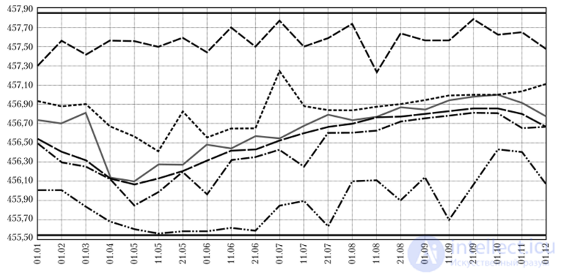
Fig. 9.6. Graphs of the six parameters considered over all 22 periods of the year at one of the found target points of the Pareto—Edgeworth set, corresponding to the values of the eight criteria yx = 0.86, y2 = y' = yA = y6 = y1 = 0, y5 = 0.77, yn = 0.93, in the reservoir cascade problem
The graphs illustrate not the front in criterion space, but namely the Pareto—Edgeworth set in the space of alternatives. The results presented in Fig. 9.6 demonstrate the fact that optimal solutions are often not smooth functions and may have noticeable kinks and jumps.
Overall, the analysis of practical applications of computer modeling of the Pareto front allows the following recommendations to be given.
Note!
For constructing and approximating the Pareto—Edgeworth set when there are three or more criteria, it is advisable to apply computer modeling and numerical algorithms (grid-based, «naive», adaptive, etc.). At the same time, even the theoretically best possible approximation of the Pareto front has a substantial error, whose asymptotic estimate for N grid nodes (6(PL., Py) ~ cosh^Y 2/(;”_,) as N —»? °°) increases sharply with an increase in the number m of criteria. Therefore, for the approximation it is advisable to use the most accurate and efficient numerical algorithms, which include four kinds of genetic algorithms, including the methods VEGA (Vector Evaluated Genetic Algorithm), EEGA (Fonseca and Fleming’s Multiobjective Genetic Algorithm), NPGA (Niched Pareto Genetic Algorithm) and SPEA (Strength Pareto Evolutionary Algorithm).
Combining numerical methods with the geometric interpretation and visualization of the Pareto—Edgeworth set provides the DM with the best possibilities for decision-making.

Comments