
Lecture
The set of criteria of a multi-criteria DMP, on the one hand, makes it possible to characterize an object from different sides; however, on the other hand, it creates an additional difficulty for making a well-founded decision, since the set of real vectors is unordered. A generalized criterion of a DMP is a criterion that reduces all the estimates for the individual criteria to a single numerical estimate.
Definition
The generalized criterion of a multi-criteria DMP is a criterion having an objective (criterial) function <p: Y —? 9?, that assigns to each vector estimate of the DMP y = (y1, y2,..., ym) ∈ Y some numerical value such that the following relation holds:

Here the criterial function is called the utility function (value function) of the multi-criteria DMP.
A sufficient condition for the existence of a generalized criterion is the condition of continuity of the preference relation. In this connection, the lexicographic preference relation, often used in practice, is unsuitable for constructing a generalized criterion because of the absence of continuity.
Note!
In practical problems, Pareto dominance is used as the preference relation by which the generalized criterion is constructed.
For a generalized criterion, what matters is not the specific value of the objective function, but the comparison of these values for different vector estimates of the DMP.
Therefore criteria will be divided into classes of equivalent criteria.
Definition
Generalized criteria with utility functions φ, and φ2 are called equivalent, if for any vector estimates y = (y1, y2,ym) and y = (y{, y2,..., ym) the following relation holds:

Example of equivalent utility functions. Suppose that for a two-criterion DMP the generalized criterion with a utility function has the form φ(y1, y2) = yx + 2yT Then the generalized criteria with utility functions φ1(yx, y2) = 3yx + 6y2 and φ2(yx, y2) = ey'+2y2 will be equivalent to it.
Generally speaking, any generalized criterion with a utility function of the form T = g°φ, where g — is an arbitrary non-decreasing function, will be equivalent to the generalized criterion with utility function φ (here the sign ° denotes composition of functions). In particular, criteria of the form T = axp, where a — is a constant, are equivalent to φ.
Since the criterial function is interpreted as the utility function of a multi-criteria DMP, the further development of the theory will proceed in accordance with the ordinalist (ordinal) approach developed by V. Pareto , who proposed considering not the utility itself of goods or bundles, but a preference ranking of some goods relative to others derived empirically. The main analytical tool in such problems became the indifference curves proposed by F. Edgeworth.
Suppose for simplicity that there are only two criteria with estimates y1 ∈ Y, and y2 ∈ Y2 respectively.
Definition
An indifference curve is the name given to those combinations of criteria values yx ∈ Y, and y2 ∈ Y2, which satisfy the equation φ(y1, y2) = c, where φ — is some constructed utility function, and c — is a given constant.
Let us consider two equally-valued points, i.e. lying on one and the same indifference curve, points A(y1> y2) and B(y1, y2) and denote Δy1 = y1 - y1, Δy2 = y2 - y2. In moving from point A to point B, for an improvement in the value of yx by | Δy11 the DM is willing to «pay» by a worsening of the value of y2 by | Δy2 (Fig. 8.2).
Note!
For points lying on one indifference curve, the quantities yx and y2 always have opposite signs.
The positive number  will depend on both points A and B. For
this dependence on point B, to be eliminated, let us consider an infinitesimally small displacement.
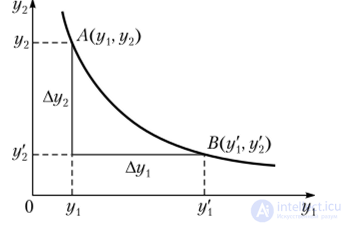
Fig. 8.2. Movement of a point on an indifference curve
Definition
The local rate of substitution (LRS) at point A(y1, y2) is the name given to the positive number

if such a limit exists and is finite.
Note!
The local rate of substitution X depends on the coordinates of point A, i.e. X = = X(y1, y2).
Strictly speaking, the LRS can be found as follows. Since the indifference curve is given by the equation <p(y1, y2) = c, where c — is a constant, in the case when the function (p(y1, y2) — is continuously differentiable, this equation can be rewritten as follows
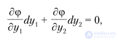
where 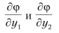 — are the partial derivatives with respect to yx and y2 respectively. Then
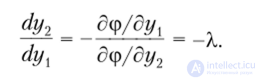
Fig. 8.3 shows the geometric meaning of the LRS: the LRS at point A(y1, y2) is equal, taken with a minus sign, to the tangent of the angle of inclination to the 0y2 axis of the tangent line drawn to the indifference curve at point A(y1, y2).
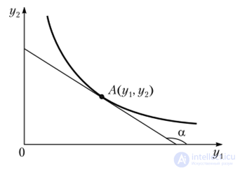
Fig. 83. Geometric meaning of the LRS: X = -tan(x
An indifference curve can be constructed for each value of the criterial function. Moreover, it follows from the definition that through any point A(y 1, y2) there passes a unique indifference curve. Thus, for the DMP we have a set of such curves.
Definition
The set of indifference curves of a certain two-criterion DMP is called an indifference map.
Fig. 8.4 shows the indifference map of a DMP with a set of vector estimates Y.
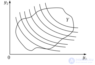
Fig.. 8.4. Indifference map
Note!
In the case where the indifference curves are smooth functions, i.e., having derivatives at every point, specifying the DMP's indifference map is equivalent to specifying, for each point A ∈ Y, its LSC.
Indeed, if an indifference map is given, then for each point A ∈ Y there exists a unique indifference curve passing through it. Drawing a tangent to the curve at this point, we find the tangent of the angle of inclination of this tangent line to the abscissa axis. This is precisely the LSC (see Fig. 8.3).
Conversely, if at every point A(y1, y2) ∈ Y the corresponding LSC is given, this means that at every point the tangent of the angle of inclination of the tangent line to the indifference curve is given. In this case the curve itself can also be constructed.

Comments