
Lecture
As an example of a decision-making problem under conditions of probabilistic uncertainty, let us consider the problem of constructing an optimal investment portfolio.
Suppose there are n securities, characterized by their returns. The return of the i-th security when a unit of capital is invested in it is described by a random variable, i = 1, 2, ..., n. The returns of individual securities are, in general, not independent random variables. Thus, there is a random vector ξ = (ξ1, ..., ξn), the characteristics of which are determined by the state of the financial market. Each specific realization of it, i.e., the resulting set of returns, is precisely a realization of the state of the environment.
A unit of capital is invested in these securities such that yi, is its share invested in the i-th type of security. An investment portfolio y is the set of numbers y1,y2,...., yn, satisfying the condition y1+ y2 +... + yn = 1. Note that some yi may be zero, meaning that capital is not invested in this particular security, or negative, meaning a short sale of the security without cover.
The decision-making problem in this case consists in constructing an investment portfolio, i.e., determining how the unit of capital should be distributed among the securities. The alternatives here will be specific portfolio values, i.e., specific sets of capital allocated among the available securities.
The result of the decision on forming an investment portfolio will be its return — a random variable

To solve the problem of constructing an optimal investment portfolio, it is necessary to construct a decision rule that determines, for what set of capital shares y1 y2,yn, such that y1 + y2 + ... yn = 1, the result (portfolio return) will be the best. Let us denote D = {y: y1 + y2 + ... + yn = 1}.
Let us consider several approaches to solving this problem. First, let us consider extremal optimization by utility.
By definition, the utility of the portfolio return is the number
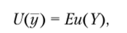
where u — is some non-decreasing function. Let us assume that u(t) = t for all real numbers t ∈ ℝ. Then the utility will be the mathematical expectation of the portfolio return
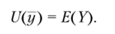
The most preferable will be such a set of capital shares y * = {y1*, y2*,..., yn*}, at which the average value of the portfolio return will be maximal

Note that, by the properties of mathematical expectation, E(Y) = y1·E(ξ1) + y2 ·E(ξ2) + ... + yn·E(ξn). Thus, to construct an optimal investment portfolio using this approach, it is not necessary to know the distribution laws of the returns of the securities included in the portfolio. It is sufficient to estimate only their mean values. However, this approach has a number of drawbacks, since it estimates only mean values and does not take into account possible deviations of returns from them, although such deviations can be quite significant.
To determine the utility of the portfolio return, other types of the function u can also be chosen, for example, u(t) = 1 - exp(-a t) , where a > 0 — some given parameter. Then the most preferable will be such a portfolio y* = (y1*, y2*,..., yn*), such that

The drawback of this approach is the complexity of its application. In particular, it is necessary to determine the exact distribution law of the vector ξ = (ξ1, ξ2,..., ξn) of the securities' returns.
Let us consider another way of constructing a decision rule for solving the problem of finding the optimal investment portfolio — extremal optimization by risk measure.
The most common measure of risk is the variance of the random variable

Then the most preferable will be such a portfolio y* = (y1*, y2,..., yn*), at which the average deviation of the investment portfolio's return from its mean value will be minimal: 
To find the variance of the portfolio's return, it is necessary to know the variances of the returns of the securities included in it, as well as their pairwise covariances, i.e., E{(ξi - E(ξj))} for all i, j ∈ {1, 2,..., n}. It is not necessary to know the actual distribution laws of the securities' returns. This simplifies the solution of this problem.
In general, different approaches to the solution can produce different and even opposite results. The choice of a particular method of solution remains up to the decision maker .

Comments