
Lecture
Decision tables (or solution tables) — are a concise visual representation for determining which actions should be performed depending on given conditions. These are algorithms , the result of which is a set of actions. Information expressed in decision tables can also be represented in the form of decision trees or, in a programming language, as a series of if-then-else and switch-case statements .
Decision tables are typically divided into four quadrants, as shown below.
| Conditions | Condition alternatives |
| Actions | Action entries |
In the simplest case, here Conditions — is a list of possible conditions, Condition alternatives — is a combination of the fulfillment and/or non-fulfillment of the conditions from this list. Actions — is a list of possible actions, Action entries — is an indication of whether or not the corresponding action should be performed for each of the combinations of conditions.
There need not be just two condition alternatives, yes or no, but several — for example, a color can be red, orange, or blue. In more complex tables, fuzzy logic may be applied.
Actions can be elementary or refer to other decision tables. The action entries can be unordered, as in this example, or ordered. In the latter case, if for a certain combination of conditions several actions can be performed, then the decision table indicates their priority.
Each decision corresponds to a variable, relation, or predicate, the possible values of which are listed among the condition alternatives. Each action represents a procedure or operation that needs to be performed, and the entries indicate whether (and in what order) the action should be performed for the set of condition alternatives to which the entry corresponds.
To make them more concise, many decision tables include a don't-care symbol in their condition alternatives . This can be a dash or a space , although the use of a space is not recommended, since this may simply indicate that the decision table is not finished. One application of decision tables is to identify conditions under which certain input factors have no bearing on the actions that need to be taken, which makes it possible to skip these input tests and thereby simplify the decision-making procedures.
Besides the basic four-quadrant structure, decision tables vary greatly in how they represent the alternatives for conditions and actions. Some decision tables use simple true/false values to represent condition alternatives (similar to if-then-else), other tables may use numbered alternatives (similar to switch-case), and some tables even use fuzzy logic or probabilistic representations for condition alternatives. Similarly, action entries may simply represent whether an action should be performed (mark the actions that need to be performed), or, in more complex decision tables, the sequence of actions that need to be performed (numbering of the actions that need to be performed).
A decision table is considered balanced or complete , if it includes all possible combinations of input variables. In other words, balanced decision tables prescribe actions for every situation in which the input variables occur. [
A limited-entry decision table is the easiest to describe. The condition alternatives are simple Boolean values, and the action entries are checkmarks indicating which actions in a given column must be performed.
The following balanced decision table is an example in which a technical support company draws up a decision table so that technical support staff can efficiently diagnose printer problems based on symptoms described to them over the phone by their customers.
| Rules | |||||||||
|---|---|---|---|---|---|---|---|---|---|
| Conditions | Printer prints | No | No | No | No | Yes | Yes | Yes | Yes |
| Red light is blinking | Yes | Yes | No | No | Yes | Yes | No | No | |
| Printer is recognized by the computer | No | Yes | No | Yes | No | Yes | No | Yes | |
| Actions | Check the power cable |  |
— | ||||||
| Check the printer-to-computer cable | |
|
— | ||||||
| Make sure the printer software is installed | |
|
|
|
— | ||||
| Check/replace the ink | |
|
|
— | |||||
| Check for a paper jam | |
|
— |
This is just a simple example, and it does not necessarily correspond to the reality of printer troubleshooting. Nevertheless, it demonstrates how decision tables can scale to multiple conditions with many possibilities.
|
|
|||||||||||||||||||||||||||||||||||||||||||||||||||||||
| The tables shown above convey identical information, but the second table uses a hyphen for brevity as the don’t-care symbol. |
Decision tables, especially when combined with the use of a domain-specific language , allow developers and policy experts to work with the same information, the decision tables themselves.
Tools for mapping nested if statements from traditional programming languages into decision tables can also be used as a debugging tool.
Decision tables turned out to be easier to understand and review than code, and they are widely and successfully used to create specifications for complex systems.
In the 1960s and 1970s, a number of languages based on decision tables, such as Filetab , were popular for business programming.
Decision tables can be, and often are, embedded in computer programs and used to «control» the program’s logic. A simple example might be a lookup table , containing a range of possible input values and a function pointer to a section of code for handling that input.
| Input | Function pointer |
|---|---|
| "1" | Function 1 (initialization) |
| "2" | Function 2 (process 2) |
| "9" | Function 9 (termination) |
In a similar way, several conditions can be encoded to encapsulate the entire logic of a program in the form of an «executable» decision table or control table . In practice there may be several such tables, operating at different levels and often linked to one another (either by pointers or by an index value).
Decision tables, also known as decision matrices or utility matrices, are a tool used for the systematic analysis and comparison of alternative options before making a decision. They help take into account various factors and their relative importance in decision-making.
Decision tables can be useful tools in the software testing process. They help with the selection of test scenarios, the prioritization of defects, and decisions about product quality. Here are a few examples of the application of decision tables in testing:
Selection of test scenarios: Decision tables can be used to assess and compare various alternative test scenarios. The criteria can be functional coverage, priority, complexity, or frequency of use of functions. Using the table, each scenario can be assessed against each criterion and a decision made as to which scenarios should be included in the test plan.
Prioritization of defects: When defects are found during testing, decision tables can help in prioritizing their correction. The criteria can be the severity of the defect, its impact on functionality, and its frequency of occurrence. Assessing each defect against these criteria makes it possible to determine which defects should be fixed first.
Assessment of product quality: When deciding on the release of a product or a particular version of it, decision tables can help in assessing quality. The criteria can be functionality, stability, performance, security, etc. Assessing the product against each criterion makes it possible to evaluate its overall readiness for release.
It is important to develop appropriate criteria and their rating values, and to ensure objectivity when filling in the table. Using decision tables helps to systematize the decision-making process in testing and to improve the quality of the decisions made.
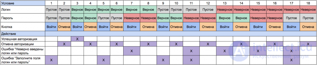
The best-known decision table similar to this is the analytic hierarchy process (AHP), the Analytic Hierarchy Method (AHM), developed by Thomas Saaty. AHM is a methodology in which a decision is broken down into a series of steps, including defining the goal, identifying alternatives, defining criteria, and comparing them with one another.
An example of a simple decision table might look as follows:
| Alternative | Criterion 1 | Criterion 2 | Criterion 3 |
|---|---|---|---|
| Option 1 | Value 1 | Value 2 | Value 3 |
| Option 2 | Value 4 | Value 5 | Value 6 |
| Option 3 | Value 7 | Value 8 | Value 9 |
Each alternative is evaluated against each criterion using the corresponding values. Various analysis methods, such as the weighted sum, can then be applied to obtain final scores for the alternatives and make a decision.
There are also other methods and approaches to decision tables, such as linear weighting methods, the TOPSIS method (technique of order preference by similarity to the ideal solution) Technique for Order of Preference by Similarity to Ideal Solution (TOPSIS) and others. The choice of a specific method depends on the context and complexity of the problem being solved.

Comments