
Lecture
For a DMP under conditions of probabilistic uncertainty, the set on which the binary preference relations are defined is the set of all possible real-valued distribution functions T (see (7.1)), described in Section 7.5.
Definition
For distribution functions D C ∈ 4x it is said that E dominates 6 (P>{ C) with respect to the first-kind stochastic dominance relation (or first order), if

moreover, for at least one value ? ∈ 9? this inequality is strict.
This means that the graph of the distribution function D(?) lies to the right of the graph of the function 6(0 (Fig. 7.2).
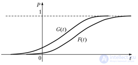
Fig. 7.2. First-kind stochastic dominance
Attention!
If F(t) — is the distribution function of the random variable ?, and G(t) — is the distribution function of the random variable ts, then by definition F(t) = P{?, = P{?> ∈ (-°°, 0} and G(t) = P{ts = P{g| g (-°°, 0}- Then the relation F(t) < G(t), Vi ∈ S.H means that the probability that the values ^ belong to the interval (-°°, i), does not exceed the probability that the values g belong to the same interval.
Example of stochastic dominance. Let us denote by P — the distribution function of the random variable. Let a > 0 — be some constant. Then p+d stochastically dominates P — Pc+D >, Fi (Fig. 7.3). For example, if ?, — is the amount of profit obtained by some store during a month, then, having increased the profit by a given non-random number of conventional units, we obtain that the probability that the profit value ?, + a is less than any given value ? does not exceed the probability that the value % is less than this value ?. In other words, the greater the profit, the less likely it is to take on small values.
Example of stochastic dominance, if P?(x) = 1 - exp(-X, x) — is the exponential distribution function with parameter X > 0, then Px >, PX] for X1 > X2 (Fig. 7.4).
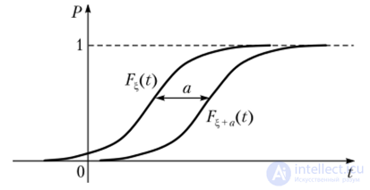
Fig. 7.3. Example of stochastic dominance
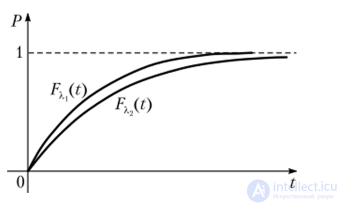
Fig. 7.4. Stochastic dominance when the distribution functions vary exponentially
If the distribution functions intersect (Fig. 7.5), then it cannot be asserted that one of the functions dominates the other with respect to the first-order stochastic dominance relation.
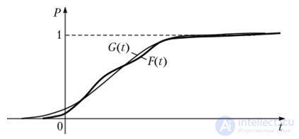
Fig. 75. Violation of the first-kind stochastic dominance property
In this case, one can consider the so-called cumulative distribution function, i.e., one can compare the areas under the distribution functions.
Definition
For distribution functions G. C, ∈ T it is said that P dominates C (/-’ 2*,, C) with respect to the second-kind stochastic dominance relation (or second order), if
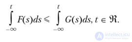
Note that first-order stochastic dominance implies second-order stochastic dominance, i.e., it is a stronger property.
Attention!
Stochastic dominance relations do not possess the property of completeness.

Comments