Features of the structure of the Pareto–Edgeworth set; the preference cone and its geometric interpretation

Geometric considerations make it possible to briefly formulate the algorithm for narrowing down the set of alternatives X demonstrated above using examples: all dominated alternatives should be discarded, leaving only the dominant ones. First of all, it is necessary to make sure that the resulting set P(X) will not turn out to be empty.

Note!

For the Pareto front (i.e., the image P(X)) not to be an empty set, it is sufficient that two conditions be satisfied:

• • the set Y must be compact (closed and bounded);
• • there must exist a nonzero vector ?, all of whose components are non-negative, and a number K such that for all y from the set Y the following holds: Y y e Y: 5 • y < K.

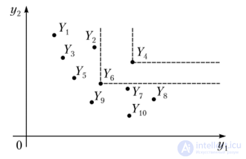
Fig. 93. Angles of preference for points Y4 and Y6 of the discrete set of possible estimates Y in the two-dimensional criterial space 9?“ and the Pareto — Edgeworth set

preference with a vertex at point Ye contains the point Y4 (see Fig. 9.3). Hence, the alternative x6, having the estimate Yb, can be excluded from the Pareto — Edgeworth set.

The points Y,, Y2, Y4 and Y8 remaining after the exclusion of all dominated alternatives represent the image of the Pareto — Edgeworth set P(X), consisting of the alternatives xp x2, x4 and x8 (see Fig. 9.3).

Let us consider the construction of the Pareto — Edgeworth set in the case of four criteria using an economic example concerning the study of the activity of a certain firm. It is not possible to use the angle of preference here, since with four criteria what needs to be constructed in four-dimensional space is no longer the angle of preference but its multidimensional analogue - the cone of preference.

Example: construction of the Pareto — Edgeworth set with four criteria present. Analysis of the quality of the products manufactured by the firm showed that in recent years the firm's product had begun to lose ground to similar products of competitors. The firm investigated the factors determining its competitiveness in order to find out which of them had begun to negatively affect the firm's competitive capabilities; the production technology, its organizational level, claims and suggestions regarding the products manufactured, trends in scientific and technological progress in the production of this product, and the quality of the raw materials, supplies, components, and information delivered to the firm were investigated.

It turned out that the technology and the organization of production and labor met the requirements of competitiveness. A more detailed analysis revealed the most «critical bottleneck». This component — the factor reducing the firm's competitiveness — turned out to be the key component part of the product.

The firm does not have the potential or the time to independently manufacture such items of the required class and quality. Therefore, at the second stage of the analysis, the market for items of this class was studied, and three of the best quality variants, manufactured by other firms and capable of ensuring, through this component part, the high quality and competitiveness of the product being manufactured, were identified. The most important parameters of the alternative decision variants for improving product quality are given in Table 9.1. It is required to select the Pareto-optimal decision variants from the four alternatives (including variant 0 — leave everything as it is, under which losses from defects amount to 4000 monetary units per year).

Table 9.1

Parameters of the alternative decision variants for improving product quality

To solve the problem, it is enough to compare the four vectors pairwise, including the three columns of Table 9.1, and the vector of estimates of the «zero» variant (in which nothing needs to be changed), having indicators of 100 (price), 0 (costs), 4000 (losses), and 1,00, respectively. When comparing, it must be taken into account that the second and third indicators (costs and forecast losses), in accordance with the remark at the beginning of the chapter, must be multiplied by (-1) so that their maximization is required in accordance with the DM's goals. Then variant 3 turns out to be dominated, since it is inferior to variant 2 on all four particular criteria. Consequently, the Pareto — Edgeworth set consists of three variants: the «zero» one (which has superiority in the second indicator — costs) and variants 1 and 2.

Let us return from the discrete set of alternatives (the example with four criteria present) to the closed region (the example of a region as a set of alternatives). The application of the angle of preference for constructing P(X) for a region as a set of alternatives is illustrated in Fig. 9.4.

Although it is not possible to construct the angle of preference at every point of the region under consideration, the successive exclusion from the set Y of its main parts makes it possible to determine P(X) fairly quickly.

At the first step, all interior points of the set Y are excluded, since the intersection of a neighborhood of any interior point M with the angle of preference constructed at that point (see Fig. 9.4) is a non-empty set. Consequently, the points of this set will be dominant with respect to the vertex M, and it cannot be the image of a point of the Pareto — Edgeworth set.

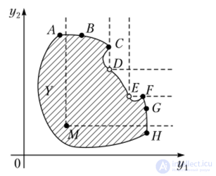
Fig. 9.4. Angles of preference for points D, E> M of the region of possible estimates Y in the two-dimensional criterial space and the corresponding Pareto front

Note!

The image of the Pareto—Edgeworth set of the region of alternatives X consists entirely of boundary points of the corresponding region of vector estimates Y. This is precisely why it is called the Pareto front (or Pareto boundary).

At the second step, after discarding all interior points, those boundary points of the set Y are excluded at which the local normal vector has at least one non-negative component.

In Fig. 9.4, these will be all points of the segments AB, AH and CH (except the points A and C), as well as, partially, the points of the segments CG) and EP. These points will be dominated by the nearest boundary segments falling within the preference angle.

At the third step, boundary points of the set Y are excluded that are dominated by remote boundary points falling within the preference angle. In Fig. 9.4, these are the remaining parts of the segments CO and EG (including the points O and E), dominated by the points C and E respectively.

Note!

Although the original region X and the region of possible estimates Y are connected sets, the Pareto front is not, i.e., it consists of three separate segments.

Thus, ultimately, the Pareto—Edgeworth set for the example (the region as the set of alternatives) consists of all points x, corresponding to the Pareto front: the curvilinear boundary segments BC, FG (including the endpoints B, C, T, C) and OE (not including the endpoints O and E).

From Fig. 9.4 it is easy to see an essential feature of the structure of the Pareto front (and hence of the Pareto—Edgeworth set): under any, arbitrarily small, rotation of the region Y, noticeable (not small) segments are added to the Pareto front. When rotated clockwise, the segment AB is added, and when rotated counterclockwise — the segment CYa. Such behavior characterizes the instability of the Pareto—Edgeworth set.

Note!

The Pareto—Edgeworth set and the Pareto front are unstable with respect to small transformations, including linear transformations of the criteria space.

This statement applies not only to the case of the region Y shown in Fig. 9.4, but also to the discrete situation.

Note!

The instability of the Pareto—Edgeworth set and the Pareto front with respect to small (including linear) transformations of the criteria space in the discrete case can lead to a sharp change in the numbers of alternatives discarded and remaining in the Pareto—Edgeworth set.

For example, suppose the set of possible vector estimates Y has not the form of a region but of a discrete set consisting of the points A, B, C, and seven more points located on the segment AB between the points A and B. Then it is easy to establish that the Pareto front contains only two points: B and C, since all points of segment AB, including the alternative A, are dominated by the option B. However, rotating the set Y in the criteria space by any, arbitrarily small, angle clockwise (which corresponds to a small linear transformation of the criteria) immediately leads to all 10 points ending up in the Pareto—Edgeworth set (i.e., their number increases fivefold), since none of the 10 points can be recognized as dominated.

Figure 9.4 demonstrates another important feature of the Pareto—Edgeworth set: linear optimization methods, including the widely used simplex methods, are unsuitable for constructing it.

Note!

Simplex methods construct only efficient vertices, i.e., vertices of a convex polytope, whereas the Pareto—Edgeworth set, even in the linear case, may turn out to be non-convex. Consequently, the set of vertices does not give a complete picture of its structure.

In Fig. 9.4, the segment BE represents that (quite significant) part of the Pareto—Edgeworth set which cannot be found by simplex methods, since, by the very structure of the algorithm, it will always be ignored by them. Meanwhile, in practice, it is precisely on this segment that the vector estimate of an alternative that is optimal for the DM may turn out to lie.

Summarizing all the conclusions drawn, it can be concluded that the geometric interpretation of the Pareto—Edgeworth set and the Pareto front by means of the preference angle makes it possible to clearly demonstrate their structure.

Note!

A simplified geometric interpretation makes it possible to visually represent both the process of finding the Pareto—Edgeworth set P(X), and the results obtained in a two-criterion efficiency decision-making problem. The features of the structure of the Pareto—Edgeworth set and its image in the criteria space — the Pareto front — are manifested in their instability with respect to small transformations (including linear ones) of the criteria space, the disconnectedness of P(X) (even for connected original sets of alternatives and their vector estimates), and the impossibility of finding it by linear methods — in particular, by the widely used simplex methods.

Note that problems similar to those considered in the example for four criteria and in Fig. 9.4 can also be solved in another way — by reducing the number of criteria through the aggregation of individual partial criteria. Historically, the first such technique was the «cost—effectiveness» method.