Lecture
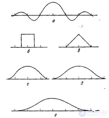
In fig. 4.3.4 shows examples of one-dimensional interpolation functions. As already noted, the function  provides accurate restoration, but, as a rule, it is difficult to form it in a real image reproduction system. The simplest interpolation function is a rectangular function, which is used to interpolate samples with a zero-order polynomial. The triangular function provides linear interpolation of the first order. Such a function can be considered as a convolution of two rectangular functions. Convolution of a triangular function with a rectangular gives a bell-shaped interpolation function, shown in Fig. 4.3.4, d. By repeating this process, one can quickly arrive at the Gaussian interpolation function shown in Fig. 4.3.4, e. Second-order and higher-order polynomials are also suitable for interpolating samples. Cubic B-spline is especially convenient for interpolating images, since interpolation results in a function that is continuous and smooth at interpolation nodes.

Fig. 4.3.4. One-dimensional interpolation functions: a -  ; b - rectangular; c - triangular (convolution of two rectangular functions); (d) bell-shaped (convolution of three rectangular functions); d - cubic B-space (convolution of four rectangular functions); e - Gaussian
The cubic B-spline is defined by [14]
 (4.3.1)
Where

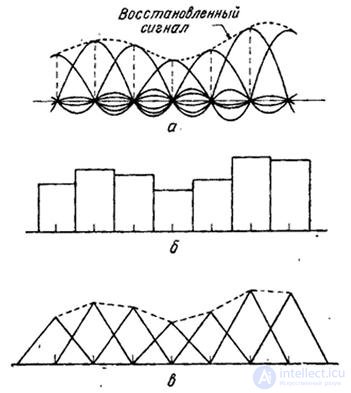
This nonzero function on only four sampling intervals can be obtained by performing convolutions of four rectangular functions. Fig. 4.3.5 illustrates the process of one-dimensional interpolation using functions  as well as rectangular and triangular functions.
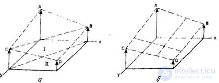
In tab. 4.3.1 the definitions of several two-dimensional separable interpolation functions are given, for which  . It should be noted that the operation of two-dimensional linear interpolation (or interpolation by first-order polynomials), similar to the operation of one-dimensional linear interpolation (Fig. 4.3.5, c), differs from interpolation using two-dimensional triangular functions presented in Table. 4.3.1. This operation should be performed in a piecewise linear fashion, as shown in Fig. 4.3.6, a. In area I, samples are linearly interpolated by the plane defined by points A, B and C, while in area II they are linearly interpolated by the plane specified by points B, C and D. The continuous bilinear interpolation method illustrated in Fig. 4.3.6, б, is reduced to sequential linear interpolation between pairs of points located on straight lines parallel to the coordinate axes. As a result, a certain surface is formed that passes through the points A, B, C and D (see Fig. 4.3.6, b). As a rule, this surface is non-planar.

Fig.4.3.5. One-dimensional interpolation: a - function  ; b - rectangular functions (interpolation of zero order); c - triangular functions (first order interpolation).
Table 4.8.1. Two-dimensional separable interpolation functions
|
Function |
Definition |
 |
|
|
Rectangular |
|
|
Triangular |
|
|
Bell shaped |
|
|
Cubic V-spline |
|
|
Gaussian |
|

Fig. 4.3.6. Two-dimensional linear interpolation: a - piecewise linear interpolation; b - bilinear interpolation.
Comments
To leave a comment
Digital image processing
Terms: Digital image processing