
Lecture
History has it that the Greek philosopher Thales (Fig. 1.1) observed the action of electric forces more than twenty-five centuries ago: he discovered that amber, when rubbed with woolen flannel, is able to attract light objects. Amber — in Greek «elektron» — gave us the term «electricity».
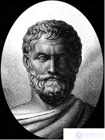
Fig. 1.1. Thales (625–547 BC) — ancient Greek philosopher and scientist
The ancient Greeks were also familiar with the special properties of iron ore (magnetite, or lodestone), which is a natural magnet. The word «magnet» comes from the Greek «stone from Magnesia» — after the name of a city in Asia Minor, near which a deposit of this ore was located.
The systematic study of electricity and magnetism began during the Renaissance, but it was only toward the end of the last century that physicists achieved a clear understanding of the foundations of the classical theory of these phenomena.
All bodies in nature are made up of atoms or molecules, which, in turn, consist of nuclei and electrons possessing electric charge.
Electric charge is a phenomenological characteristic of the properties of elementary particles and their interactions.
Between charged elementary particles there exist special interaction forces called electric forces. It has been established experimentally that these forces can be either attractive or repulsive; therefore, to describe electric interaction, two types of electric charges are introduced, conventionally called negative and positive: like charges repel each other, while unlike charges attract (Fig. 1.2).
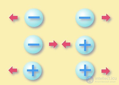
Fig. 1.2. Two negative charges repel each other, a negative and a positive charge attract each other, two positive charges repel each other
The charge of electrons is considered negative, and the charge of protons — positive. Neutrons, which are part of nuclei, carry no electric charge. Electric interaction forces bind the nucleus and electrons into a single stable system — the atom.
The smallest electric charge in magnitude experimentally found in nature is the charge of the electron. The charge of the proton is exactly equal to it in magnitude and opposite in sign:

|
The electric charge of the proton |
Note that the value of the elementary charge given above is usually used for approximate calculations and for solving school and university problems. In fact, experimental physicists have determined it with much greater precision. Currently, the tables (Journal of Physics G. Nuclear and Particle Physics. Vol. 37, No. 7A, July 2010, Article 075021) give the following value of the elementary charge

Owing to the exact equality of the magnitudes of the proton and electron charges, the total positive and negative charges in each atom are equal in magnitude, and therefore bodies are usually electrically neutral. However, by applying some effort, electrons can be torn away from some bodies, which then become positively charged, and transferred to other bodies, which become negatively charged. Such bodies are macroscopically charged. The electric charge of any body is a multiple of the elementary charge e, that is, it varies discretely:
|
|
(1.1) |
where N — is an integer. The discreteness of the possible values of electric charge is customarily referred to as the quantization of electric charge.
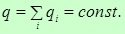
Numerous experiments have proved that the law of conservation of electric charge holds:
|
In any electrically isolated system of charged bodies, the total electric charge is conserved:
|
A physical system whose boundary surface cannot be crossed by charged particles is customarily called electrically isolated. Therefore, in many cases, in particular when deriving equations that are the integral or differential form of the law of conservation of charge, the following formulation of it is quite useful:
|
The only way to change the charge of any physical system is to introduce charged particles into the system through its boundary surface. |
Obviously, «introducing» charged particles into the system or «removing» them from the system is, in an algebraic sense, one and the same thing. Note also that a similar approach proves productive when writing other conservation laws as well: of energy, momentum, angular momentum, etc.
At the microscopic level, the law of conservation of charge follows from the analysis of reactions between elementary particles and, of course, nuclear reactions. Let us take, for example, the alpha decay of a uranium isotope (Fig. 1.3):

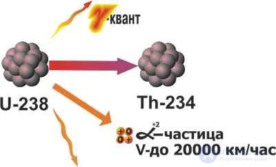
Fig. 1.3. Alpha decay of uranium-238 isotope
The atomic number Z of the uranium nucleus is 92, which means that the nucleus contains 92 protons, that is, its charge is qU = 92e. For thorium Z = 90, that is, the charge of its nucleus is qTh=90e, and for helium Z = 2 and qHe = 2e. The fulfillment of the equality

means that electric charge is conserved in this reaction. Never have reactions been observed involving nuclei or elementary particles in which the law of conservation of electric charge is violated. This does not mean that particles with electric charge cannot disappear or be created, but in that case particles with the same but opposite-sign charge must also disappear or be created. The main point is that the total charge remains unchanged before and after the reaction. As an example, let us consider the so-called annihilation reaction: an electron e– with charge –e collides with its antiparticle — the positron e+, whose charge is positive and equal to +e. As a result, two photons g are produced (Fig. 1.4).
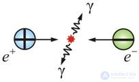
Fig. 1.4. Annihilation reaction of an electron and a positron
It is easy to verify that the reaction
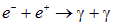
satisfies the law of conservation of electric charge: the total charge before and after the reaction equals zero. At the same time, a reaction such as, for example,

in which charge is not conserved.
The electron is the lightest of the charged particles, and owing to the law of conservation of charge (and the law of conservation of energy), it simply has nothing to decay into. Therefore the electron is stable, and this is a necessary prerequisite for the stability of atoms, molecules, matter, and of ourselves.
Let there be two charged macroscopic bodies whose dimensions are negligibly small compared with the distance between them. In this case each body can be regarded as a material point, or «point charge».
The French physicist C. Coulomb (1736–1806) experimentally established the law that bears his name (Coulomb's law) (Fig. 1.5):
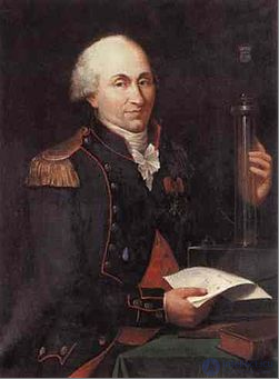
Fig. 1.5. C. Coulomb (1736–1806) — French engineer and physicist
|
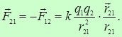
In vacuum, the interaction force between two stationary point charges is proportional to the magnitude of each of the charges, inversely proportional to the square of the distance between them, and directed along the straight line connecting these charges:
|
Fig. 1.6 shows the electric repulsive forces arising between two like point charges.
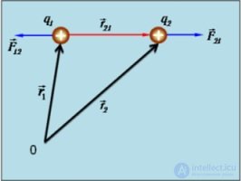
Fig. 1.6. Electric repulsive forces between two like point charges
Recall that  , where
  and
and  — are the position vectors of the first and second charges, so the force acting on the second charge as a result of its electrostatic — «Coulomb» interaction with the first charge can be rewritten in the following «expanded» form
|
|
(1.3) |
Let us note the following rule, convenient when solving problems: if the first index of the force is taken to be the number of the charge on which this force acts, and the second – the number of the charge that creates this force, then keeping the same order of indices on the right-hand side of the formula automatically ensures the correct direction of the force — corresponding to the sign of the product of the charges:  — repulsion and
  — attraction, with the coefficient
  always.
To measure the forces acting between point charges, an instrument created by Coulomb, called a torsion balance, was used (Figs. 1.7, 1.8).
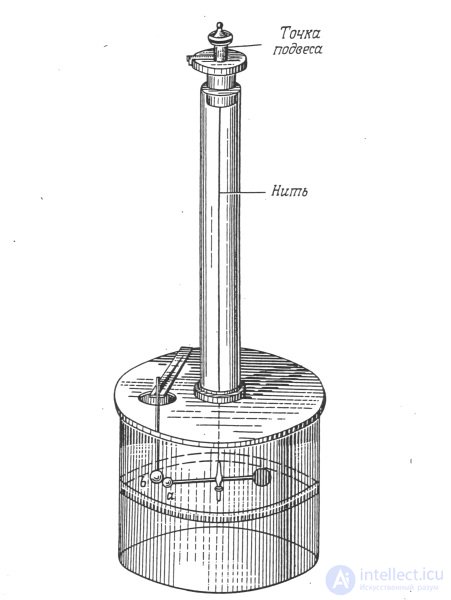
Fig. 1.7. C. Coulomb's torsion balance (drawing from a 1785 work). The force acting between charged balls a and b was measured
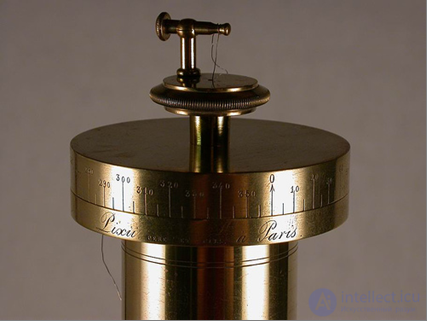
Fig. 1.8. C. Coulomb's torsion balance (suspension point)
A light beam is suspended on a thin elastic thread, with a metal ball fixed at one end and a counterweight at the other. Next to the first ball, another identical stationary ball can be placed. A glass cylinder protects the sensitive parts of the instrument from air movement.
To establish the dependence of the electrostatic interaction force on the distance between the charges, arbitrary charges are imparted to the balls by touching them with a third charged ball mounted on a dielectric handle. From the angle of twist of the elastic thread, the repulsive force of the like-charged balls can be measured, and from the instrument's scale, the distance between them.
It should be said that Coulomb was not the first scientist to establish the law of charge interaction that now bears his name: 30 years before him, B. Franklin arrived at the same conclusion. Moreover, the precision of Coulomb's measurements was inferior to the precision of experiments carried out earlier (H. Cavendish).
To introduce a quantitative measure for determining the precision of the measurements, let us assume that in reality the interaction force of the charges is inversely proportional not to the square of the distance between them, but to some other power:
 .
.
No scientist would undertake to assert that d = 0 exactly. The correct conclusion should read as follows: experiments have shown that d does not exceed...
The results of some of these experiments are given in Table 1.
Table 1.
Results of direct experiments testing Coulomb's law
|
Experiment |
Year |
d |
|
Robison |
1769 |
<0.06 |
|
Cavendish |
1773 |
<0.02 |
|
Coulomb |
1785 |
0.02 |
|
Maxwell |
1873 |
<5·10–5 |
|
Plimpton, Lawton |
1936 |
<2·10–9 |
|
Bartlett et al. |
1970 |
<1.3·10–13 |
|
Williams et al. |
1971 |
<3.0·10–16 |
Charles Coulomb himself verified the inverse-square law to within an accuracy of a few percent. The table gives the results of direct laboratory experiments. Indirect data, based on observations of magnetic fields in outer space, lead to even stronger constraints on the value of d. Thus, Coulomb's law can be considered a reliably established fact.
In SI, the unit of current (the ampere) is a base unit, and consequently the unit of charge q turns out to be a derived one. As we shall see later, the current I is defined as the ratio of the charge  flowing through the cross-section of a conductor during a time
  to this time:

From this it is evident that the magnitude of a steady current is numerically equal to the charge flowing through the cross-section of a conductor per unit time, and accordingly:
|
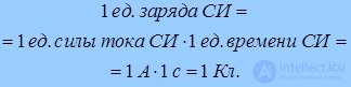
In SI, the unit of measurement of electric charge is the coulomb (C) — the electric charge that flows in 1 second through the cross-section of a conductor at a constant current of 1 A:
|
The proportionality coefficient in Coulomb's law is written as:
|
|
(1.4) |
With this form of writing, the experiment yields the value of the quantity  , which is customarily called the electric constant. The approximate numerical value of the electric constant is as follows:
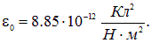
Since most often enters equations in the combination

let us give the numerical value of the coefficient  itself

As in the case of the elementary charge, the numerical value of the electric constant has been determined experimentally with high precision:

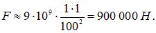
The coulomb is too large a unit for practical use. For example, two charges of 1 C each, placed in vacuum at a distance of 100 m from each other, repel each other with a force
For comparison: a body of the following mass presses on the ground with the same force
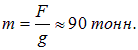
This is approximately the mass of a freight railroad car, for example, loaded with coal.
The superposition principle is a statement according to which the resulting effect of a complex process of action is the sum of the effects caused by each action separately, provided that the latter do not mutually influence one another (Physical Encyclopedic Dictionary, Moscow, «Soviet Encyclopedia», 1983, p. 731). It has been established experimentally that the superposition principle holds for the electromagnetic interaction considered here.
In the case of the interaction of charged bodies, the superposition principle manifests itself as follows: the force with which a given system of charges acts on some point charge is equal to the vector sum of the forces with which each charge of the system acts on it.
Let us illustrate this with a simple example. Suppose there are two charged bodies acting on a third with forces  and
and  respectively. Then the system consisting of these two bodies — the first and the second — acts on the third body with a force

This rule is valid for any charged bodies, not only for point charges. The interaction forces of two arbitrary systems of point charges are calculated in Appendix 1 at the end of this chapter.
It follows that the electric field of a system of charges is determined by the vector sum of the field strengths created by the individual charges of the system, i.e.

Adding the electric field strengths according to the rule of vector addition expresses the so-called superposition principle (independent superposition) of electric fields. The physical meaning of this property is that an electrostatic field is created only by charges at rest. Consequently, the fields of different charges «do not interfere» with one another, and therefore the total field of a system of charges can be calculated as the vector sum of the fields from each of them separately.
Since the elementary charge is very small, while macroscopic bodies contain a very large number of elementary charges, the distribution of charge over such bodies can in most cases be regarded as continuous. In order to describe exactly how the charge is distributed over a body (uniformly, non-uniformly, where there is more charge, where there is less, etc.), let us introduce charge densities of the following three kinds:
· volume charge density  :
:
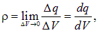
where dV — is a physically infinitesimal element of volume;
· surface charge density  :
:
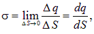
where dS — is a physically infinitesimal element of surface;
· linear charge density  :
:
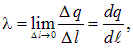
where  — is a physically infinitesimal element of line length.
Here and throughout,  is the charge of the physically infinitesimal element under consideration (of volume, of a surface patch, of a line segment). By a physically infinitesimal portion of a body, here and below, is meant such a portion of it which, on the one hand, is so small that under the conditions of the given problem it can be regarded as a material point, while, on the other hand, it is so large that the discreteness of the charge (see relation ) of this portion can be neglected.
General expressions for the interaction forces of systems of continuously distributed charges are given in Appendix 2 at the end of the chapter.
Example 1. An electric charge of 50 nC is uniformly distributed over a thin rod 15 cm long. On the extension of the rod's axis, at a distance of 10 cm from its nearest end, there is a point charge of 100 nC (Fig. 1.9). Determine the force of interaction between the charged rod and the point charge.
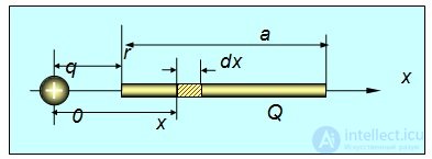
Fig. 1.9. Interaction of a charged rod with a point charge
Solution. In this problem the force F cannot be determined by writing Coulomb's law in the form or (1.3). Indeed, what is the distance between the rod and the charge: r, r + a/2, r + a? Since, under the conditions of the problem, we have no right to assume that a << r, applying Coulomb's law in its original formulation, valid only for point charges, is impossible; it is necessary to use the standard technique for such situations, which is as follows.
|
If the interaction force of point bodies is known (for example, Coulomb's law) and it is necessary to find the interaction force of extended bodies (for example, to calculate the interaction force of two charged bodies of finite size), then these bodies must be divided into physically infinitesimal portions, the known relation for each pair of such «point» portions must be written, and, using the superposition principle, the sum (integral) over all pairs of these portions must be taken. |
It is always useful, if not to say necessary, before proceeding to the concretization and performance of the calculation, to analyze the symmetry of the problem. From a practical point of view, such an analysis is useful in that, as a rule, given a sufficiently high symmetry of the problem, it sharply reduces the number of quantities that need to be calculated, since it turns out that many of them are equal to zero.
Let us divide the rod into infinitesimal segments of length  , the distance from the left end of such a segment to the point charge being equal to
  .
.
The uniformity of the distribution of the charge  over the rod means that the linear charge density
  is constant and equal to
 ,
,
Consequently, the charge  of the segment
  is equal to
 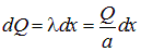 , whence, in accordance with Coulomb's law, the force acting on the point charge q as a result of its interaction with the point charge
  , is equal to

As a result of the interaction of the point charge q with the entire rod, a force will act on it
|
|
(1.5) |
Substituting the numerical values here, for the magnitude of the force we obtain:

From (1.5) it is seen that at  , when the rod can be regarded as a material point, the expression for the interaction force of the charge and the rod, as it should, takes the usual form of Coulomb's law for the interaction force of two point charges:
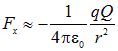
Example 2. A ring of radius  carries a uniformly distributed charge . What is the force of interaction between the ring and a point charge q located on the axis of the ring at a distance
  from its center (Fig. 1.10).
Solution. By the condition, the charge is uniformly distributed over a ring of radius . Dividing by the circumference, we obtain the linear charge density on the ring 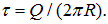 Let us isolate an element of the ring of length
  . Its charge is equal to
 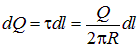 .
.
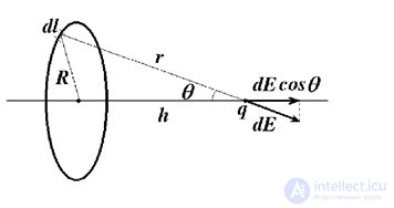
Fig. 1.10. Interaction of a ring with a point charge
At point q this element creates an electric field
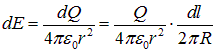
We are interested only in the longitudinal component of the field, since when summing the contribution from all elements of the ring, only it is nonzero:
|
|
Integrating over  , we find the electric field on the axis of the ring at a distance
  from its center:
|
|
|
From this we find the required force of interaction of the ring with the charge q:
|
|
|
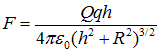
Let us discuss the result obtained. At large distances from the ring  , the quantity of the ring's radius under the radical sign can be neglected, and we obtain the approximate expression

This is not surprising, since at large distances the ring looks like a point charge  and the interaction force is given by the ordinary Coulomb's law. At small distances the situation changes sharply. Thus, when a test charge q is placed at the center of the ring
  , the interaction force is zero. This is also not surprising: in this case the charge q is attracted with equal force by all elements of the ring, and the action of all these forces mutually cancels.
Since the electric field is zero both at  and at
  , somewhere at an intermediate value
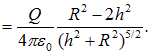
  the electric field of the ring is maximal. Let us find this point by differentiating the expression for the field strength E with respect to the distance
|
|
|
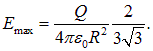
Setting the derivative equal to zero, we find the point  where the field is maximal. At this point it is equal to
Example 3. Two mutually perpendicular infinitely long threads, carrying uniformly distributed charges with linear densities  and
and  , are located at a distance a from each other (Fig. 1.11). How does the interaction force between the threads depend on the distance a?
Solution. Let us first discuss the solution of this problem by the method of dimensional analysis. The interaction force between the threads may depend on the charge densities on them, the distance between the threads, and the electric constant, that is, the sought formula has the form:
|
|
|
where  is a dimensionless constant (a number). Note that, owing to the symmetric arrangement of the threads, the charge densities on them can enter only in a symmetric way, to equal powers. The dimensions of the quantities entering here are known in SI:
|
|
|
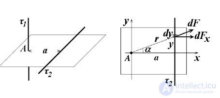
Fig. 1.11. Interaction of two mutually perpendicular infinitely long threads
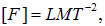
Compared with mechanics, a new quantity has appeared here — the dimension  of electric charge. Combining the two preceding formulas, we obtain an equation for the dimensions:
|
|
|
Equating the powers of M and T on both sides of this equation, we immediately obtain  There is no quantity of charge dimension on the left-hand side, whence it follows that
  or
or  Finally, equating the powers of the length dimension, we obtain the equation
  whence it follows that
  Finally we have:
|
|
|
Thus, it turns out that the interaction force between the threads does not depend on the distance between them. Recall that the dimensionless constant C cannot be determined by the method of dimensional analysis. In essence we have already obtained the answer to the problem, but let us also give its exact solution, which will allow us to find C. In Fig. 1.11, on the right, a top view is shown of the plane containing the thread  point A marks the intersection of the drawing plane with the thread
  . The electric field strength created by the thread at the point where the element
  of the second thread is located, is equal to
|
|
|
On the element of the thread a force acts
|
|
|
We are, however, interested only in the component 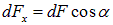 of this force along the axis
  , since the longitudinal component is compensated exactly by the same force acting on the symmetric element of the thread below. Let us express all distances in terms of the angle
  :
:
|
|
|
We finally obtain the expression for the component of the force acting on the element 
|
|
|
Integrating this expression over the angle  from
from  to
to  , we find the total force acting on the thread:
|
|
|
We have again confirmed that the force between the threads in this problem does not depend on the distance  between them. Moreover, this time we have determined the dimensionless constant:
Around every electric charge there always exists an electric field.
|
The electric field created by a stationary charge (or a system of stationary charges) is called electrostatic. |
Interaction between charges is carried out by means of the electrostatic field. The very concept of a field has proved to be very fruitful and is widely used in modern physics. The appearance of a field means that something has changed in the space surrounding us. Mathematically, a field is described by a quantity that varies from point to point. For example, one can consider the velocity field in a flowing fluid. At each point of the volume of the fluid a velocity vector is given, which may vary with time (unsteady flow) or may be constant (steady flow). This is an example of a vector field. The field of stationary electric charges belongs to the same type of field.
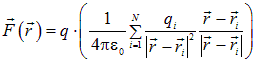
Let us write the expression for the force acting on a point charge  as a result of its interaction with a system of point charges
  (relation from Appendix 1)
|
|
(1.6) |
Here  is the position vector of the point at which the charge
  is located. The charge , on which the force acts, is sometimes called the «test» charge in such situations, and is written out as a separate factor. The expression standing in parentheses is determined exclusively by the properties of the system of charges that acts on the charge . Naturally, this action (force) depends on where it is located; accordingly, the expression in parentheses depends on the position vector , which determines the location of the charge . Following the idea, presented above, of the electrostatic field existing around every charge and, of course, system of charges, let us introduce a force characteristic of this field, called the strength of the electric field.
|
The electric field strength is called the vector
|
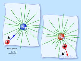
Fig. 1.12. Field strength vector of a negative and a positive point charge
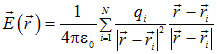
From the definition of field strength it follows that the field strength of an arbitrary system of charges at rest can be written in the form
|
|
(1.8) |
Indeed, the force with which a given system of charges acts on a point charge is equal to the vector sum of the forces with which each charge of the system acts on it. It follows that the electric field strength of a system of charges is determined by the vector sum of the field strengths created by the individual charges of the system. The so-called superposition principle (independent superposition) of electric fields holds
|
The field strength created by a system of stationary charged bodies is equal to the vector sum of the field strengths created by each body separately:
|
The superposition principle is one of the most general principles of modern physics. Let us emphasize that field strengths add vectorially.
Fig. 1.13 illustrates the superposition principle of fields using the example of a field created by two point charges.
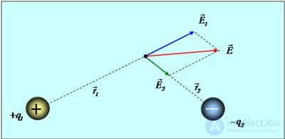
Fig. 1.13. Superposition principle of electric fields
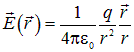
For a single charge  , located at the origin
  , for the field strength it creates at a point with position vector
  , we obtain (index 1 omitted):
|
|
(1.9) |
The field strength of a point charge at different points of space is, in general, different both in magnitude and direction (Fig. 1.14). The field of a point charge is a central field; the center of symmetry of the field coincides with the point at which the charge is located.
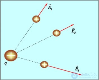
Fig. 1.14. Electric field strength vectors of a charge q at different points of space
|
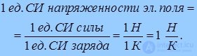
In SI, the unit of measurement of electric field strength is the newton per coulomb (N/C), — that is, the unit of field strength is taken to be the strength of such a field in which a force of 1 N acts on a charge equal to 1 C:
|
In practice, another name for this unit is more often used — «volt per meter» (V/m) (the unit «volt» will be discussed a little later).
Typical values of electric field strengths encountered in our world are given in Fig. 1.15.
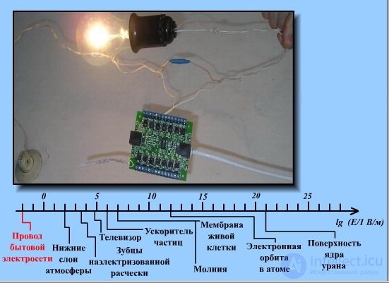
Fig. 1.15. Typical values of electric field strengths encountered in nature
Let us note the similarity between Coulomb's law and the law of universal gravitation
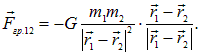
The role of charges is played by masses, and the gravitational constant G is analogous to the coefficient 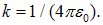 The minus sign corresponds to the fact that gravitational interaction is always attractive. One can also introduce a gravitational field strength vector as the ratio of the force
  , for example, to a test mass
  :
:
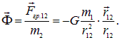
If here  — is the mass of the Earth, and
  its radius, then
  is nothing other than the well-known acceleration of free fall
  m/s2 (up to a very small centrifugal force of inertia included in the force of gravity
  )
)

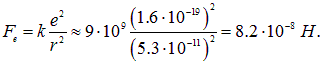
Example 4. The average distance between the electron and the proton in a hydrogen atom is r = 5.3·10–11 m (Fig. 1.16). Find the electrostatic  and gravitational
  attractive forces between them and determine the ratio of these forces.
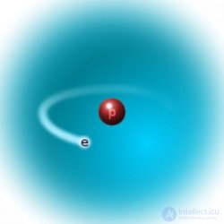
Fig. 1.16. Electron and proton in a hydrogen atom
Solution. From Coulomb's law we have
In turn, from the law of universal gravitation it follows that

The ratio of the forces  does not depend on the distance between the electron and the proton and is equal to
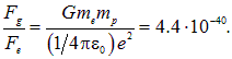
This calculation shows that at the scale of atoms and molecules, gravitational forces are so much smaller than electrostatic ones that they can be neglected.
So why is it that in the macroscopic world we inhabit, we become acquainted with the law of gravity after our very
продолжение следует...
Часть 1 1. The electric field in vacuum
Часть 2 1.4. Flux of a vector. The Ostrogradsky–Gauss theorem for a
Часть 3 1.5. Application of Gauss's theorem for calculating the electric field
Часть 4 Appendices - 1. The electric field in vacuum
Часть 5 - 1. The electric field in vacuum
 , is called the elementary charge.


















 , equal to the ratio of the force acting on a point charge
  to the algebraic value of this charge (Fig. 1.12)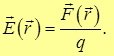


Comments