
Lecture
All bodies in nature can be conditionally divided, according to their electrical properties, into two large categories — conductors, which readily pass electric current, and insulators (dielectrics), which practically do not pass current. The term «dielectric» was introduced by M. Faraday. The division of substances into conductors and dielectrics according to their ability to conduct current is fairly arbitrary. In strong electric fields even good dielectrics pass electric current. However, there exist substances, called semiconductors, that actually occupy an intermediate position in conductivity between conductors and dielectrics. Their distinguishing feature is a rapid rise in conductivity as temperature increases. Recall that the conductivity of metals decreases as temperature rises. Semiconductors will be examined in the second volume. For now we are interested in the behavior of conductors placed in an electrostatic field.
The electrical properties of bodies depend on their internal structure. Thus, in metals under ordinary conditions there are many «free» electrons that have detached from the ions of the crystal lattice and move almost unimpeded throughout the volume of the metal. In the absence of external fields the motion of free electrons is completely chaotic. Switching on an arbitrarily small external electric field causes directed motion of the electrons. Substances of this kind, in which under ordinary conditions there are quite a lot of «free» charge carriers, are called conductors (Fig. 2.1).
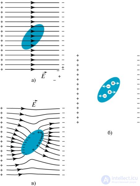
Fig. 2.1. a) the body is neutral and non-conducting, so its positive and negative charges are immobile; b) the free charges of a conducting body begin to move; c) after the motion stops, an equilibrium state is established
In the absence of an external electric field, the free charges inside an uncharged conductor are in equilibrium. This means that the charge carried by the «free» electrons through any cross section of the conductor is on average equal to zero. Thus, inside and outside an isolated uncharged conductor the average field, and hence the average charge density, are equal to zero.
We are now interested in the answers to three questions. What happens if an excess charge is imparted to an isolated conductor? What happens if an isolated uncharged conductor is placed in an external electric field? Finally, what are the properties of a system of charged conductors?
If part of the electrons is added to (or removed from) a conductor, it becomes negatively (positively) charged. Let us consider the conditions for the equilibrium of charges on a conductor. In equilibrium there is no directed motion of charges inside the conductor. This means that the field inside the conductor is zero:  . Otherwise
  the charges would have to move. Since inside the conductor
  , then by the Ostrogradsky-Gauss theorem, at every point in the volume of the sample
  , so the volume charge density inside the conductor is also equal to zero
 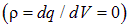 , and the excess charges can be located only on the surface of the conductor. This occurs because like charges repel one another and tend to be arranged as far apart as possible.
Let us answer the question: what happens if there is a closed internal cavity within a charged conductor? Will charges also be arranged on its walls? Based on qualitative considerations, we must answer no: the charges, repelling one another, will be arranged only on the outer surface of the conductor. The Ostrogradsky — Gauss theorem leads to the same conclusion. If we take an imaginary surface that lies entirely within the thickness of the conductor and is infinitely close to the walls of the cavity, then at every point of this surface the field is zero, and consequently the flux of the electric field strength vector is also zero. Hence there are no charges on the walls of the cavity.
The absence of a field inside a charged conductor means that the potential inside it is constant: since 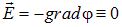 , then
  . Thus the potential on the surface of the conductor is also constant and equal in magnitude to the potential in the bulk of the conductor. Consequently, the surface of a conductor is equipotential (Fig. 2.2).
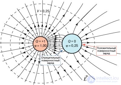
Fig. 2.2. Potentials of two conductors: the left conductor has a charge of +1 (in arbitrary units), the right conductor is uncharged. The potentials are constant throughout the volume of each conductor
Electric charges located on the surface of a conductor with some density  create an electric field outside the conductor. Near the surface of the conductor the field strength is directed along the normal
  at every point of the surface, i.e.
  since the equipotential surface is perpendicular to the field lines. To calculate the field near the conductor we again use the Ostrogradsky — Gauss theorem. As the imaginary surface let us take the surface of an infinitesimally small cylinder positioned perpendicular to the conductor so that one of its bases lies outside the conductor and the other — inside (Fig. 2.3).
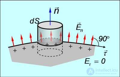
Fig. 2.3. Electric field near the surface of an isolated charged conductor
In this case the flux through the base inside the conductor is zero, since there is no field inside the conductor. Next, the flux through the side walls is also zero, since they are parallel to the field strength vector. What remains is the flux through the base of area  outside the conductor.
Then the total flux of the electric field strength vector  through the surface of the cylinder will be equal to:
|
|
(2.1) |
According to the Ostrogradsky — Gauss theorem,
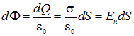
whence
|
|
(2.2) |
Thus, the electric field strength near the surface of a charged conductor (on its outer side) is proportional to the surface charge density. Inside the conductor, recall, the field is zero.
See.
Distribution of charges over the surface of a conductor in equilibrium conditions.
Electric wind.
Franklin's «plasma engine».
Problem. Studies of atmospheric electricity have shown that near the Earth's surface there exists a stationary electric field with an average strength of  . This field is directed downward. Note that during a thunderstorm the distribution of atmospheric electricity has a more complex character (Fig. 2.4).
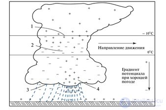
Fig. 2.4. Distribution of atmospheric electricity in a mature thunderstorm cell: 1 — center of positive charges, 2 — center of negative charges, 3 — rain with negative charge, 4 — center of positive charge in the region of heavy rain
Using this data and assuming that the Earth is a conductor, estimate the total electric charge of our planet.
Solution. First let us determine the sign of this charge. Since the field is directed downward, toward the Earth, and field lines begin on positive charges and end on negative ones, we conclude that the Earth's charge is negative. Next, from equation (2.2) we find:

Knowing the Earth's radius  km, we determine the area of the Earth's surface
  m2 . Finally, we find the electric charge of the Earth
  kC!
kC!
When an uncharged conductor is placed in an external electric field, the free charges begin to move and after a short time reach equilibrium. A stationary distribution of charges is established, in which an excess of negative charge forms on one side of the conductor, and an excess of positive charge on the other. This phenomenon is called electrostatic induction (Fig. 2.5).
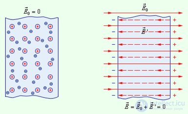
Fig. 2.5. Electrostatic induction
The field of the induced charges (which appear on the surface of the conductor) completely cancels the external field inside the conductor. Otherwise, electric charges would be moving inside the conductor, and the distribution would not be stationary. Thus, in the equilibrium state, the total field (external plus that of the induced charges) inside the conductor is zero. Therefore, the conclusions we drew earlier for charged conductors in the absence of an external field also hold for the total field.
In particular, there will be no electric field in the internal cavity within the material of the conductor (Fig. 2.6). The property of conductors to shield external fields (preventing them from penetrating into the region enclosed by the conductor) is the basis of electrostatic protection against the action of external electrostatic fields (Fig. 2.7).
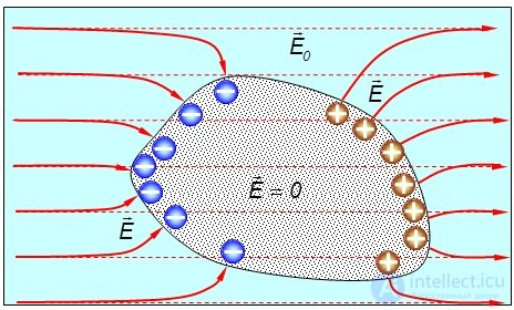
Fig. 2.6. Appearance of induced charges on the surface of a conductor
under the action of an external electric field 
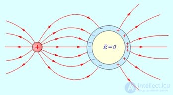
Fig. 2.7. Electrostatic shielding. The field in the metal cavity is zero
Thus, a car is a safe shelter during a thunderstorm, and not because the rubber on its wheels insulates it from the ground. Here we must be grateful to the Ostrogradsky — Gauss theorem. However, it should be emphasized that a closed hollow conductor shields the cavity inside it only from external charges and fields. If charges are introduced inside the cavity, an electric field will appear there, while the field in the conductor itself will still be zero.
Further, the total field near the conductor is perpendicular to its surface and is equal to
|
|
(2.3) |
where  — is the density of the induced charges (we assume that the conductor as a whole is uncharged).
In practice, one has to solve the following problem. A certain external field is given. A conductor of a given shape is introduced into it. One needs to find the distribution of the charges induced on it and the resulting changes in the total field outside the conductor. The charge density at a given potential of the conductor is determined by the curvature of the surface:  increases with increasing positive curvature (convexity) and decreases with increasing negative curvature (concavity) (Fig. 2.8).
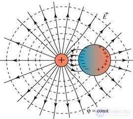
Fig. 2.8. Electric field (field lines and equipotential surfaces)
of an uncharged sphere near a point electric charge
Problem. Given a spherical metal shell with inner and outer radii  and
and  respectively. A charge
  is placed at the center of the cavity. Find the electric field and potential of the system, as well as the distribution of charges on the surface of the shell (Fig. 2.9).
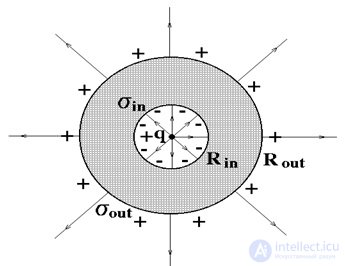
Fig. 2.9. Electric field of a positive charge  surrounded by a metal shell
Solution. Owing to spherical symmetry, the charges will be arranged on the surfaces of the shell with a constant surface density:  — on the inner and
  — on the outer sides. Let us first consider the field inside the shell. Let us draw an imaginary spherical surface of radius
  Inside it there is only the charge
  . Consequently, the field in the cavity of the shell will be the same as for an isolated charge. Let us now take a surface of radius
  , where
  . Since there is no field in the metal, the flux through our surface is zero. This means that the total charge inside it is zero. It consists of the charge and the total charge on the inner surface, which must therefore equal
  . On the other hand, the charge on the inner surface can be determined as
  , from which it follows that
 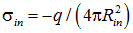 . The metal shell as a whole was uncharged, so the total charge that appeared on its inner surface must be compensated by the total charge
  that arose on the outer surface of the shell (conservation of electric charge). Therefore the charge density
 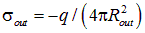 . Finally, let us draw an imaginary surface outside the metal shell
  . The total charge inside the surface consists of 1) the charge
  , 2) the charge on the inner surface of the shell, and 3) the charge on its outer side. Therefore the charge inside the imaginary surface is
  . This means that the electric field outside the shell again coincides with the field of a single point charge . Thus we have established that the electric field is directed along the radius vector
  and in absolute value is equal to
|
|
(2.4) |
It remains for us to find the field potential at various points of the system. Outside the shell the potential coincides with the potential of a point charge:  On the outer surface of the shell the potential equals
  Since there is no field inside the shell, the potential retains this value at all points inside the metal. Inside the cavity the potential again coincides with the potential of a point charge. Since the latter is defined up to a constant, we have
  The value of this potential on the inner surface of the shell
  must coincide with the value of the potential
  on the outer shell. From this we can find the constant
We finally obtain:
|
|
(2.5) |
Graphs of the field strength and potential as functions are shown in Fig. 2.10.
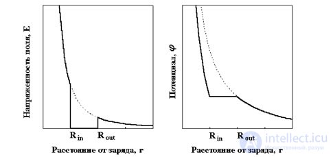
Fig. 2.10. Field strength and potential of the electric field of a charge q,
surrounded by a metal shell with inner radius  and outer radius
The dashed lines correspond to the characteristics of the field of a single charge in the absence of the shell
Energy can be stored by lifting a weight (a cuckoo clock), winding a spring (an ordinary mechanical watch), or compressing gas (an air gun). Energy can also be stored in the form of an electrostatic field. Devices called capacitors serve this purpose. In the crudest approximation, any capacitor is a pair of conductors (plates) between which a certain potential difference  is created. The ability of a capacitor to store energy in the form of an electrostatic field is characterized by the value of its capacitance. This term itself dates back to the time when there existed a notion of an electric fluid. Let us imagine a vessel that we fill with such a fluid. Its level (the difference in height between the bottom of the vessel and the surface of the fluid) corresponds to the potential difference
  to which the capacitor is charged. And the amount of fluid in the vessel corresponds to the charge
  imparted to the capacitor. Depending on the shape of the vessel, at the same level (potential difference) more or less fluid (charge) will enter it. The ratio
  is called the capacitance of the capacitor.
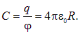
Isolated conductors also possess capacitance. The role of the second plate is played in this case by points at infinity. Consider, for example, a charged sphere of radius  . Outside the sphere
  there is a Coulomb electric field
|
|
(2.6) |
directed along the radius. The potential created by the charged sphere at  is given by the expression
|
|
(2.7) |
Inside the conducting sphere  , and consequently the potential is constant at all points of this sphere and coincides with the value of the potential on its surface:
|
|
(2.8) |
This value is essentially the potential difference between the surface of the sphere and a point at infinity. By the definition of capacitance
|
|
(2.9) |
In SI the unit of capacitance adopted is the farad (in honor of M. Faraday): a farad is the capacitance of a conductor which, to raise its potential by 1 V, must be given a charge of 1 C:

The relation for the capacitance of an isolated sphere in vacuum  shows that 1 F is the capacitance of a ball with radius
  m, which is 13 times the radius of the Sun and 1413 times the radius of the Earth. Thus the capacitance of the Earth is approximately 1/1413 F, i.e.
  μF. In other words, 1 F is an enormous capacitance. The manufacture of capacitors of such capacitance has only been mastered relatively recently, mainly owing to improvements in the technology of depositing ultrathin dielectric and metal films. For example, the overall size of a 1 F capacitor made by NEC/TOKIN (www.nec-tokin.net/now/english/index.html) is less than 22 mm, and its mass is 6.7 grams.
An increase in the capacitance of a conductor can be achieved not only by increasing its dimensions, but also by bringing another conductor close to it. Examples are the parallel-plate capacitor, the spherical capacitor, and others. We will calculate their capacitances based on the given definitions and the geometry of the capacitor.
Parallel-plate capacitor (Fig. 2.11).
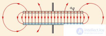
Fig. 2.12. Electric field of an ideal parallel-plate capacitor
An ideal parallel-plate capacitor consists of two metal parallel plates whose linear dimensions are much greater than the distance  between them. Let the area of each plate be equal to
  (Fig. 2.12). A charge
  is placed on one plate, and
  — on the other. If the plates are large enough, they can be considered «infinite» in the sense that it is permissible to neglect «edge» effects — the charge distributions and field configurations near their edges.
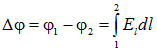
Then the charges are distributed over the inner surfaces of the plates practically uniformly, with a constant density. The potential difference between the plates equals the integral of the field strength, taken along any path between them:
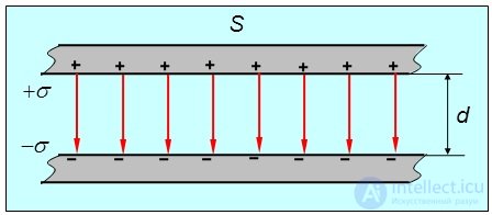
Fig. 2.12. Electric field of an ideal parallel-plate capacitor
Then the charges are distributed over the inner surfaces of the plates practically uniformly, with a constant density  . The potential difference between the plates equals the integral of the field strength, taken along any path between them:
|
|
(2.10) |
The field created by two infinite parallel planes charged oppositely with equal densities is uniform, and its strength equals  (see (2.3)).
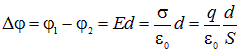
The field strength in the space surrounding the plates can be taken as equal to zero, if edge effects are neglected. Integrating along a field line (which are orthogonal to the plates), we obtain
|
|
(2.11) |
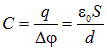
From this we find the capacitance of a parallel-plate capacitor:
|
|
(2.12) |
Cylindrical capacitor. A cylindrical capacitor consists of two long coaxial conducting cylinders of radii  and
and 
 and length
  . Assuming that
  , we again neglect edge effects in this case. The linear charge density on the cylinders equals
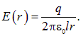
  . We have already derived the expression for the electric field of a long charged cylinder (see (1.17)):
|
|
(2.13) |
The electric field is directed along the radius of the cylinders. Integrating along this path from one plate to the other, we find the potential difference between the plates:
|
|
(2.14) |
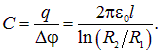
From this follows the expression for the capacitance of a cylindrical capacitor:
|
|
(2.15) |
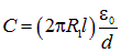
In the case when the gap between the plates  , one can use the first term of the Taylor series expansion of the logarithm
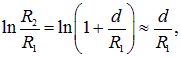
which leads to the expression
|
|
(2.16) |
In parentheses stands the product of the circumference of the cylinder and its height, which equals the surface area of the cylinder (the area of the plates). Thus, in this limit we have reproduced expression (2.12) for the capacitance of a parallel-plate capacitor.
Spherical capacitor. A spherical capacitor is formed by two concentric spheres of radii  and
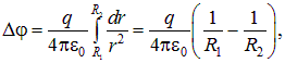
and  . Integrating along the radius the now-familiar expression
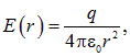
we obtain the potential difference between the plates:
|
|
(2.17) |
whence
|
|
(2.18) |
If the outer radius is infinitely large  (physically this means that
  ), then the subtracted term in the denominator can be neglected, and we arrive at formula (2.9) for the capacitance of an isolated sphere. In the opposite case, when
  the gap between the plates, we can set in the numerator
  Noting that
  is the area of the plates, we again arrive at formula (2.12).
Problem. A capacitor used in a computer memory chip has a capacitance of  and is charged to a potential difference
  . What is the number
  of excess electrons on its negative plate? In what mass of water is the total number of all atomic electrons equal to ?
Solution. The charge of the capacitor equals  . To find the number of excess electrons, one must divide
  by the charge of the electron:
  Almost two million electrons — is this a lot or a little? To find out, let us find the mass of water with the same number of electrons. A water molecule
  contains two atoms of
  and one atom of
  , that is, 10 electrons in total. Hence, the mass of water we are interested in must contain
  molecules. The number of molecules in one mole equals
  that is, we must take
  mole. The molar mass of water equals
 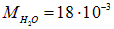 kg/kmol, so the sought mass amounts to
  kg, that is, extremely small. A million particles — a lot in the world of electrons, but very little on the scale of our world.
Series connection
In many cases, to obtain the required capacitance, capacitors are combined into a group called a battery. The capacitance of a battery of capacitors depends on the scheme by which the capacitors comprising it are connected. Two types of connection are distinguished: series and parallel. A mixed type of connection of capacitors into a battery is also possible.
|
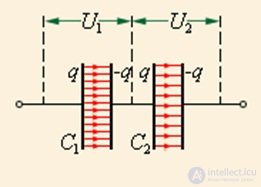
Fig. 2.13. Series connection of capacitors Series connection. When the battery is charged (Fig. 2.13), the potential difference is distributed among the individual capacitors and will equal
If a charge The potential differences
On the other hand,
where
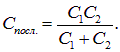
For a battery of two capacitors, for example, this yields the expression (Fig. 2.14)
|
Parallel connection
|
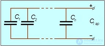
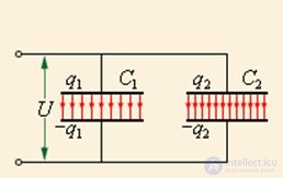
Fig. 2.15. Parallel connection of capacitors In a parallel connection of capacitors (Fig. 2.15) the potential difference of the battery equals the potential difference of each individual capacitor:
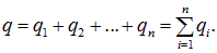
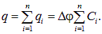
By charging such a battery, we impart to it a charge, part of which will end up on the plates of the first capacitor, part — on the plates of the second, and so on. As a consequence of the law of conservation of electric charge, the total charge of a battery of parallel-connected capacitors will equal the sum of the charges of the individual capacitors:
For each capacitor one can write the relation
substituting which into (2.25), we obtain:
On the other hand,
where
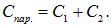
that is, for a parallel connection of capacitors the capacitance of the battery equals the sum of the capacitances of the individual capacitors. For a battery of two capacitors, for example, this yields the expression (Fig. 2.16)
Fig. 2.16. Parallel connection of two capacitors Problem. Into a spherical capacitor with an inner sphere radius of
Fig. 2.17. A spherical capacitor with a conducting shell inside it can be represented |
Solution. The capacitance  of the original capacitor, whose plates were spheres of radii
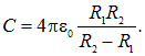
  is given by formula (2.18):
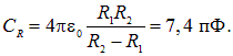
As can be seen from the figure, the new capacitor is a series connection of two spherical capacitors: one formed by spheres of radii  (its capacitance we denote as
  ) and
) and  (its capacitance will be
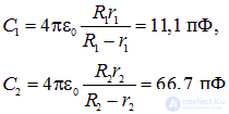
  ). Using the same formula we have:
|
|
(2.30) |
For the capacitance  of the series-connected capacitors we now obtain
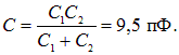
The capacitance of the new capacitor turned out to be greater than the capacitance of the original one.
The analytical formula for the capacitance of such a battery has the form:
|
|
(2.31) |
For an infinitely thin inner sphere  the charges on its surfaces would cancel each other out, and we should obtain the formula for the capacitance of a capacitor
  without the inner shell. And indeed this follows from formula (2.31) at
  . In the opposite limiting case, when the walls of the inner shell are close to the plates of the original capacitor, one obtains the formula for the capacitance of two series-connected parallel-plate capacitors.
Capacitors have found wide practical application, especially in radio engineering. Some types of capacitors are shown in Fig. 2.18.
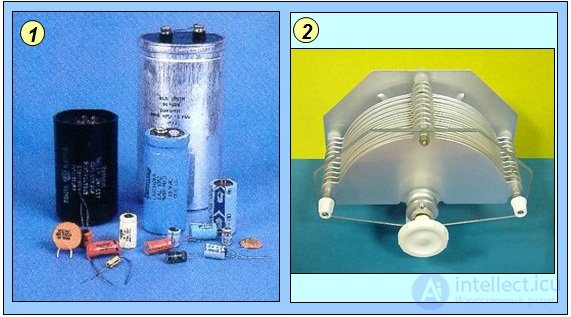
Fig. 2.18. Various types of capacitors used in engineering: 1 — fixed-capacitance capacitors; 2 — variable-capacitance capacitor
A system of charged bodies possesses potential energy. Let us first consider two charges  and
and  located at a distance
  (Fig. 2.19). As one of the charges is removed to infinity, the force of interaction between them decreases to zero.
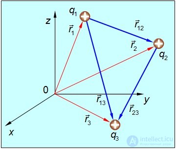
Fig. 2.19. On determining the energy of a system of electric charges
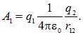
To bring the charges together to a distance  requires doing work, which goes into changing the potential energy of the system. Let a charge
  approach a charge
  from infinity to a distance
  . The work done in moving it equals:
|
|
(2.32) |
where  — is the potential of the field created by the charge at the point to which the charge is moved, i.e.
|
|
(2.33) |
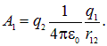
Similarly, one can consider that the charge approached from a point at infinity:
|
|
(2.34) |
The results turned out to be the same, since the final arrangement of the charges is the same. Consequently, the potential energy of interaction of two charges equals
|
|
(2.35) |
or in symmetric form
|
|
(2.36) |
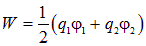
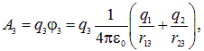
To the system of charges and , let us now add a third charge  (Fig. 2.19), transferred from infinity to a point separated from charge by a distance
  , and from charge by a distance
  . The corresponding work will be equal to:
|
|
(2.37) |
where  is the potential created by charges and at the point where charge is located.
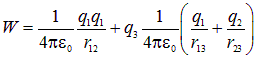
The potential energy of interaction of the three charges is equal to:
|
|
(2.38) |
Let us rewrite the resulting relation as:
|
|
(2.39) |
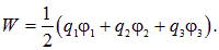
or in symmetric form
|
|
(2.40) |
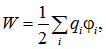
It is clear that for an arbitrary system of charges we have
|
|
(2.41) |
where  is the potential at the point where charge
  is located, created by all the other charges except
  .
.
Problem. Two like-charged particles with charges  and
and  and masses
  and
and  are launched from a great distance toward each other along the straight line connecting them, with speeds
  and
and  , respectively. Determine the smallest distance
  to which the particles can approach each other.
Solution. First, let us answer the question: why does a minimum possible distance of approach of the particles exist at all, why can they not collide with each other? The answer is simple: the particles repel each other by virtue of Coulomb's law, and the potential energy of interaction grows without bound as  . The initial kinetic energy of the particles is simply not enough to overcome the infinitely high potential barrier between them. Let us consider the process of the particles approaching each other. As the distance
  between them decreases, the repulsive forces braking the particles grow. The rate of approach — the relative velocity of the particles — decreases and at some moment becomes zero. At this instant the particles move as a single whole, their velocities are the same (we shall denote them
  ). This is precisely the moment of closest approach. Afterward, under the influence of repulsion, the particles begin to separate again and ultimately move apart from each other.
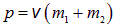
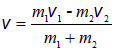
Having analyzed the process, let us turn to the equations. In the initial state the total momentum of the particles is equal to 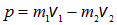 (we take the first particle to be moving in the positive direction). At the moment of closest approach the particles move with the same velocity (the velocity of their center of mass), and the momentum of the system is equal to
  . Since the total momentum is conserved, we find the velocities of the particles at the moment of closest approach:
|
|
(2.42) |
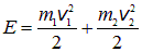
Now let us apply the law of conservation of energy. At the initial moment, when the particles are infinitely far from each other, the total energy  consists of their kinetic energies:
|
|
(2.43) |
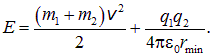
At the moment of closest approach the total energy is equal to the sum of the kinetic energies of the particles and the potential energy of their Coulomb interaction:
|
|
(2.44) |
Equating the right-hand sides of equalities (2.43) and (2.44) and substituting expression (2.42) for the velocity  , we finally obtain the relation
|
|
(2.45) |
Here 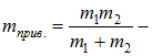 is the reduced mass of the colliding particles,
 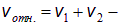 is the relative velocity of the particles, and
  is the kinetic energy of their relative motion. From (2.45) for
  we obtain:
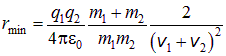
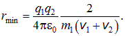
This formula can now be applied to various special cases. For example, if the masses of the particles are equal  , then from (2.45) we find
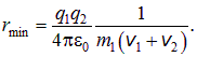
If, on the other hand, the mass of the second particle is much greater than the mass of the first  , then the minimum distance turns out to be half as large as in the case of equal masses:
A system of charged bodies possesses potential energy. Let us first consider two charges and located at a distance (Fig. 2.19). As one of the charges is removed to infinity, the force of interaction between them decreases to zero.
Fig. 2.19. On the determination of the energy of a system of electric charges
To bring the charges together to a distance it is necessary to do work, which goes toward changing the potential energy of the system. Let charge approach charge from infinity to a distance . The work of moving it is equal to:
|
|
(2.32) |
where is the potential of the field created by charge at the point to which charge is moved, i.e.
|
|
(2.33) |
Similarly, we can consider that charge approached from an infinitely distant point:
|
|
(2.34) |
The results turned out to be the same, since the final arrangement of the charges is the same. Consequently, the potential energy of interaction of two charges is equal to
|
|
(2.35) |
or in symmetric form
|
|
(2.36) |
To the system of charges and , let us now add a third charge (Fig. 2.19), transferred from infinity to a point separated from charge by a distance , and from charge by a distance . The corresponding work will be equal to:
|
|
(2.37) |
where is the potential created by charges and at the point where charge is located.
The potential energy of interaction of the three charges is equal to:
|
|
(2.38) |
Let us rewrite the resulting relation as:
|
|
(2.39) |
or in symmetric form
|
|
(2.40) |
It is clear that for an arbitrary system of charges we have
|
|
(2.41) |
where is the potential at the point where charge is located, created by all the other charges except .
Problem. Two like-charged particles with charges and and masses and are launched from a great distance toward each other along the straight line connecting them, with speeds and , respectively. Determine the smallest distance to which the particles can approach each other.
Solution. First, let us answer the question: why does a minimum possible distance of approach of the particles exist at all, why can they not collide with each other? The answer is simple: the particles repel each other by virtue of Coulomb's law, and the potential energy of interaction grows without bound as . The initial kinetic energy of the particles is simply not enough to overcome the infinitely high potential barrier between them. Let us consider the process of the particles approaching each other. As the distance between them decreases, the repulsive forces braking the particles grow. The rate of approach — the relative velocity of the particles — decreases and at some moment becomes zero. At this instant the particles move as a single whole, their velocities are the same (we shall denote them ). This is precisely the moment of closest approach. Afterward, under the influence of repulsion, the particles begin to separate again and ultimately move apart from each other.
Having analyzed the process, let us turn to the equations. In the initial state the total momentum of the particles is equal to (we take the first particle to be moving in the positive direction). At the moment of closest approach the particles move with the same velocity (the velocity of their center of mass), and the momentum of the system is equal to . Since the total momentum is conserved, we find the velocities of the particles at the moment of closest approach:
|
|
(2.42) |
Now let us apply the law of conservation of energy. At the initial moment, when the particles are infinitely far from each other, the total energy consists of their kinetic energies:
|
|
(2.43) |
At the moment of closest approach the total energy is equal to the sum of the kinetic energies of the particles and the potential energy of their Coulomb interaction:
|
|
(2.44) |
Equating the right-hand sides of equalities (2.43) and (2.44) and substituting expression (2.42) for the velocity , we finally obtain the relation
|
|
(2.45) |
Here is the reduced mass of the colliding particles, is the relative velocity of the particles, and is the kinetic energy of their relative motion. From (2.45) for we obtain:
This formula can now be applied to various special cases. For example, if the masses of the particles are equal , then from (2.45) we find
If, on the other hand, the mass of the second particle is much greater than the mass of the first , then the minimum distance turns out to be half as large as in the case of equal masses:
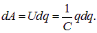
The process of charges appearing on the plates of a capacitor can be represented as though very small portions of charge  are successively taken from one plate and transferred to the other plate (Fig. 2.20). In this case we can write relations analogous to the formulas of the previous section:
|
|
(2.53) |
Here 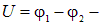 is the potential difference between the plates, and
  is the charge of the capacitor at the moment of transfer
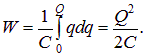
  . To charge an uncharged capacitor to some final charge
  requires that work be done
|
|
(2.54) |
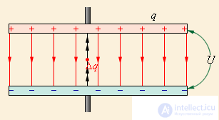
Fig. 2.20. The process of charging a capacitor
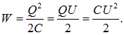
This is precisely the energy stored in the capacitor. It can also be written in the form:
|
|
(2.55) |
The choice of any of these equivalent formulas is dictated by the conditions of the problem being solved. Note also that applying the general formula (2.41) for the energy of a system of charges also leads to these expressions:
|
|
(2.56) |
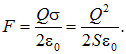
In the case of a parallel-plate capacitor, the field strength inside it does not depend on the distance between the plates. This allows us to look at the process of charging a capacitor from a different angle. Suppose that charges  already exist on the plates, which are located infinitely close to each other. The energy in such a system is zero, since the surface charges compensate each other. Let us begin to move one of the plates away. On its side, the other plate exerts a force on it equal to the product of the charge of the plate
  and the field strength
  created by the stationary plate (this field is half the total field in the capacitor):
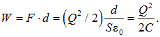
When the plates are moved apart from each other by a distance  , the work
  done is equal to the energy that will be stored in the capacitor:
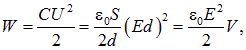
Where, then, is the energy of the electric field stored in the capacitor concentrated? To answer this question, the mental exercise we have just carried out — charging a parallel-plate capacitor by the "method" of moving the plates apart — will help us. We were doing work, the energy of the capacitor was increasing, but what was changing in the system? The charges on the isolated plates did not flow away anywhere, and the field strength inside the capacitor also did not change. The only change is the increase in the volume of space between the plates. And in that space we have nothing except the electric field. This means that in every small volume of space pervaded by field lines, some energy is concentrated. To find it, let us write the energy of a parallel-plate capacitor in such a way that the volume of space between the plates appears explicitly.
The field strength of a parallel-plate capacitor is related to the potential difference between the plates and the size of the gap  by the relation
  . Let us write the energy of the parallel-plate capacitor in the form
|
|
(2.57) |
where  is the volume of space between the plates.
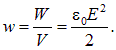
Since the field in a parallel-plate capacitor is uniform, the energy is distributed in space with a density
|
|
(2.58) |
We have obtained a formula whose significance extends far beyond problems about capacitors. In essence, capacitors are no longer visible in this formula: there is the strength of the electric field (regardless of what creates it), which determines the density of energy distribution at every point of space.
Let us demonstrate this using the example of the field of a uniformly charged sphere of radius  . As we saw above when calculating the electromagnetic radius of the electron, the energy of the electrostatic field is equal to
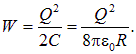
Let us obtain this same result by a different route.
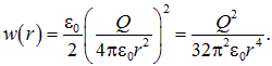
The field strength in the external space  , as we already know, is the same as for a point charge. Therefore the field energy density is equal to
|
|
(2.59) |
Let us take a point in space, specified in spherical coordinates by  , and select a small volume
  The electrostatic energy concentrated in this small volume is equal to
 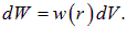 The total energy can be found by integrating
  over the entire space outside the sphere:
|
|
(2.60) |
The energy of the charged sphere obtained earlier has now been calculated from its distribution in the surrounding space! This is a very powerful result, demonstrating that the electric field is not some fiction or artificial mathematical device. It is real, it contains within itself energy that can be measured and put to use for one's own benefit. And all of this occurs in vacuum! We need conductors as a convenient storage place for electric charges, while the field and its energy are concentrated outside them. This means that, despite the absence of matter, a vacuum is not as empty as one might imagine. At the very least, we have just become acquainted with one of the forms of existence of matter, distinct from ordinary tangible substance.
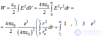
Problem. Obtain expression (2.51) for the energy of the electron, starting from formula (2.58).
Solution. Using the expression for the electrostatic energy density, we obtain, after simple integration:
|
|
(2.61) |
Naturally, we obtain the same result. Note that from our derivation it follows that most of the energy of a uniformly charged ball falls on the space surrounding it: only 16.7% of the energy is concentrated inside the ball.


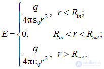
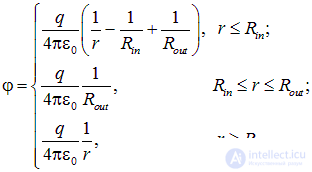



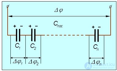

 is imparted to the first plate of the battery of capacitors, then an induced charge
  appears on its second plate. Since this plate is connected to the first plate of the second capacitor, and since the law of conservation of charge holds, a charge
  .
. ,
,  etc. may not be equal to one another, since the capacitances of the individual capacitors are, generally speaking, not the same. Therefore the potential difference across the terminals of the whole battery is found as the sum of the voltages
  across each of the capacitors: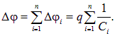
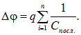
 is the capacitance of the whole battery. Consequently, the capacitance of a battery of series-connected capacitors is given by the expression: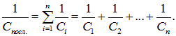



 is the capacitance of the whole battery. Comparing (2.27) and (2.28) we finally obtain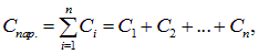
 cm and an outer sphere radius of
  cm, a solid spherical conducting shell with inner radius
  cm and outer radius
  cm was placed (Fig. 2.17). Compare the capacitances of the original and the new capacitor.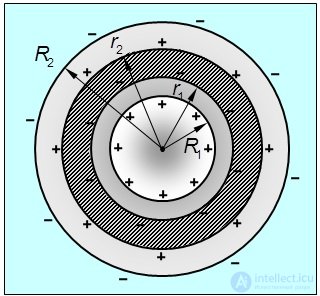








Comments