
Lecture
Now we have arrived at genuine quantum mechanics. Everything up to this point has been intuitive semiclassical notions that made it possible to incorporate ideas of quantum physics into classical physics. But this level of knowledge is insufficient for calculations, for quantitative predictions of many phenomena. A coherent system is required — a theory of the motion (or propagation) of microparticles with dual (wave-particle) properties.
The previous section ended with the statement that we have not yet established what exactly oscillates during the motion of an electron. This has happened before in the history of physics. Once, when deriving the equations of electrodynamics, Maxwell also did not know what the oscillations and waves he was describing actually represented, yet the equations turned out to be correct. So let us set aside for now the question of the physical nature of de Broglie waves and simply introduce a certain "electron" wave, that is, a wave function  . About it we know for now only one thing: the wave function must describe the results of experiments that demonstrate the wave properties of electrons (diffraction, etc.).
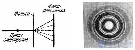
Fig. 4.1. Diffraction pattern produced by an electron beam passing through a metal foil
Video 4.1. Diffraction of electrons on a polycrystal.
Let us mentally picture V.A. Fabrikant's experiment (see Sec. 3.2), in which electrons were directed one at a time onto a crystal acting as a diffraction grating. Behind the crystal a photographic plate was placed, on which typical diffraction rings eventually appeared. From classical physics we know which mathematical tools describe such a pattern: the ordinary addition of interfering waves, whose intensities are proportional to

True, unlike an ordinary wave, an electron does not split into parts: as electrons pass through the crystal, each of them lands at some single point on the photographic plate, causing blackening right there and nowhere else. This reveals the properties of the electron as a particle. Despite identical initial conditions, electrons, as the experiment showed, land at different points. For any given electron it is impossible to know in advance exactly which point on the plate it will hit. This reveals its wave properties. A diffraction pattern arises once a sufficiently large number of such electrons have passed through the crystal. The intensity of blackening of the plate at a given point is proportional to the number of particles that landed there, that is, to the probability of landing.
In classical physics, the blackening of the plate is determined by the intensity of the wave, that is, by the squared modulus of the wave function. It turns out that the quantity

is proportional to the probability of finding the electron in the vicinity of the point  at time t. The de Broglie wave is a probability wave! A single act of interaction between the electron and the crystal remains a single act (electron-as-particle), but its outcome can only be predicted probabilistically, statistically (electron-as-wave). This is the meaning of wave-particle duality. Quantum mechanics was created in 1925–1927 by W. Heisenberg and E. Schrödinger; the probabilistic interpretation of the wave function was given a little later in the works of M. Born and the Bohr school.
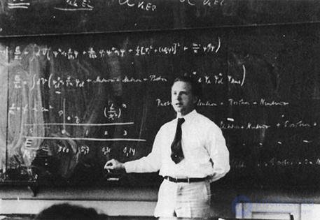
Fig. 4.2. W. Heisenberg formulated the uncertainty principle in 1927.
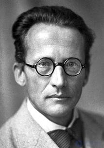
Fig. 4.3. Erwin Rudolf Josef Alexander Schrödinger (1887–1961)
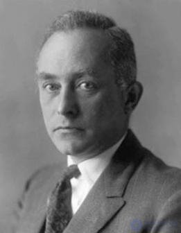
Fig. 4.4. Max Born (1882–1970)
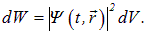
So, the probability of finding the electron in the vicinity of the point must be proportional to

But the probability of detecting the electron exactly at a given location is vanishingly small; it only makes sense to speak of it landing in a small volume  surrounding that point. It is clear that the probability
  of finding the electron there is proportional to the size of the volume. Therefore for the probability we have
|
|
|
(4.1) |
In other words

— this is the probability density of finding the particle at the point with radius vector .
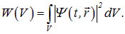
The probability  of finding the particle in some finite volume
  is computed with the help of the addition of probabilities, that is, by integration
|
|
|
(4.2) |
The integration in (4.2) is carried out over the volume (in the case of one-dimensional motion — over the segment).
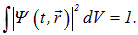
The total probability of finding the particle somewhere at all in space must equal unity. From this follows the so-called normalization condition of the wave function: the same integral over the whole of space equals unity, that is
|
|
|
(4.3) |
Remark: satisfying this condition is possible for those problems in which the classical particle moves within a bounded region of space (finite motion). For infinite (spatially unbounded) motions, the normalization condition becomes more complicated.
Observable physical quantities must be described by real numbers and functions. Accordingly, we represented classical waves (sound, electromagnetic) in the form

One could make use of the mathematical formalism of complex numbers, based on Euler's formula

where

— is the imaginary unit. Then the same wave could be represented as the real part of the expression
|
|
|
(4.4) |
where
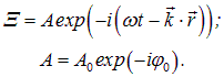
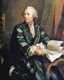
Fig. 4.5. Leonhard Euler (1707–1783)
The initial phase here is included in the complex amplitude A. When applied to classical waves, both formalisms are equivalent, since in the end only the real part of the wave is taken. Unlike classical waves, the probability wave is complex. Physical observable quantities are expressed through the squared modulus of the wave function, so that in quantum mechanics too they will be described by real numbers. But the complexity of the wave function has a deep connection with the law of conservation of electric charge, so the use of complex numbers and functions in quantum mechanics is not a whim but a necessity. The surface of constant phase in the wave  (4.4) propagates along the wave vector
  , the phase velocity of the wave is still equal to

so that the transition to complex waves does not change the relations we are used to.
The wave function is the principal object of study in quantum mechanics. Speaking of some state in classical physics, we assumed that at time t=0 the particle had a certain position and velocity (momentum), and its subsequent fate was predetermined by Newton's equations of motion.
A state in quantum mechanics has a different meaning: at time  the wave function is given, and its change is governed by an equation not yet known to us (Schrödinger's equation). In this sense causality is now understood as follows: in classical physics — exact predictions of positions and velocities; in quantum mechanics — predictions of states (wave functions). The equations of a new physics (in this case, the Schrödinger equation) are never logically derived from prior principles (otherwise it would not be a new theory, but a consequence of the old one). But the quantum-mechanical equation must have certain classical roots, since classical mechanics works well within its domain of applicability. Below we will present not a derivation, but suggestive reasoning (as in Sec. 3.3 for the uncertainty relations).
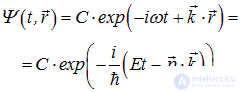
A free particle corresponds to a de Broglie wave, which we write in the form of a classical plane wave (in complex form)
|
|
|
(4.5) |
where the modulus of the wave vector k is related to the wavelength by

C — amplitude. We have already used the known relation between the energy and momentum of a particle and the frequency and wavelength of the de Broglie wave. The sought equation for the wave function must not contain  and
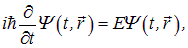
and  since these are — characteristics of a specific state of the particle. Let us try to find operations on the wave function of a free particle that allow us to eliminate the parameters and E and p. We have for the time derivative
|
|
|
(4.6) |
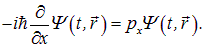
and with respect to the spatial coordinate 
|
|
|
(4.7) |
The same equations arise upon differentiating with respect to ,  and
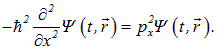
and  . Repeating the differentiation with respect to the coordinates, we obtain
|
|
|
(4.8) |
Adding (4.8) to the analogous equations for the second derivatives with respect to , and , we arrive at the relation
|
|
|
(4.9) |
where the symbol  denotes the Laplace operator:
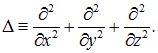
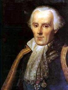
Fig. 4.6. Pierre-Simon Laplace (1749–1827)
At this point a distinction arises between the relativistic and nonrelativistic cases. The quantum mechanics considered here is a nonrelativistic theory, in which

This classical relation lets us connect the time differentiation in (4.6) with the differentiation with respect to spatial coordinates in (4.9), and thereby eliminate from the equation the dependence on the particle's energy and momentum:
|
|
|
(4.10) |
This equation would fully suit us, but so far it has been written only for a free particle. It is easy to see what the equation should look like for a system with a constant value  of the potential energy. The total energy equals the sum
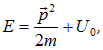
so that we obtain
|
|
|
(4.11) |
In the case of a particle located in an arbitrary potential field, near the point  the potential energy can be considered a constant quantity
  , so that the sought generalization follows almost obviously from equation (4.11):
|
|
|
(4.12) |
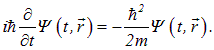
This is the fundamental equation of quantum mechanics — the famous general Schrödinger equation. Let us stress once again that it cannot be strictly derived, but it can be guessed, proceeding from suggestive reasoning. The correspondence of the equation and its consequences to physical reality is verified experimentally. The Schrödinger equation is essentially an analogue of the classical relation between the total energy  of a particle and its kinetic energy
  . For a free particle they coincide. In the presence of a potential field this relation takes the form
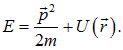
We already know that the total energy corresponds to the derivative with respect to  , the momentum components — to derivatives with respect to x,y,z, and the kinetic energy — to second derivatives with respect to the spatial coordinates, since momentum enters it to the second power. The classical potential energy, as we see, corresponds in quantum mechanics to the ordinary product of
  with the wave function.
The Schrödinger equation is linear in the sought wave function, from which the following consequences immediately follow:
|
|
So, the state of an electron is described in quantum mechanics by the wave function  . But where did the coordinates, momentum, and other quantities known from classical theory go? We must abandon classical notions. In their place we have acquired so-called operators, that is, certain operations performed on . From the Schrödinger equation we see that it reproduces the relation

of the total energy with the kinetic energy  and the potential energy
  , but the classical quantities are replaced by operators acting on the wave function
  . We shall denote an operator by the same symbol as the classical quantity, marking it with a "hat" for distinction. Then the Schrödinger equation (4.12) can be written in operator form, in which its connection with the energy relations of classical physics is clearly visible:

where the operators are introduced
|
|
|
(4.13) |
Here
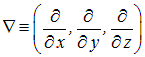
is the gradient operator, the square of which gives the Laplace operator  . The radius-vector operator
  reduces to simple multiplication of
  by the vector
  ; the same holds for any function (in particular, for the potential energy).
We have arrived at a method of passing from known classical relations to the corresponding quantum ones: the classical quantities must be replaced in them by the corresponding operators.
Rule 1
|
To the classical dynamical variables
— differentiation with respect to the coordinates. |
In this case, to the energy of a particle
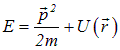
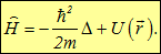
in a potential field there corresponds the total energy operator
|
|
|
(4.14) |
In these notations the Schrödinger equation (4.12) has the form
|
|
|
(4.15) |
The total energy operator is called the Hamiltonian (the analogue of the Hamiltonian function in theoretical mechanics).
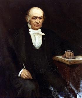
Fig. 4.7. Sir William Rowan Hamilton (1805–1865)
Recall that in classical mechanics conservation laws are connected with the symmetry of the system: energy — with translation (shift) of time

momentum — with translation of space

angular momentum — with rotations in space (translation of angles)

Translation of some generalized coordinate  is produced by the operator of differentiation with respect to that coordinate. For example, for an infinitesimal translation

we have, by the definition of the derivative

Therefore it is not by chance that in quantum mechanics the total energy corresponds to the operation of taking the derivative with respect to time

while momentum corresponds to the gradient. Similarly, the operator of the projection of angular momentum onto some axis  is proportional to the differentiation operator

with respect to the angle of rotation about that axis:
|
|
4.4. The Stationary Schrödinger EquationIn operator theory an important role is played by so-called eigenstates of operators. These are states that, under the action of a given operator, change in a trivial way: they are multiplied by some number. This number is called the eigenvalue of the operator, corresponding to the given eigenstate. To find the eigenstates and eigenvalues of some operator, one must solve the equation
where the index n distinguishes one solution from another. The set of quantities Let us consider as an example the operation of rotation about some axis
The connection between mathematics and physics is realized in the following rule. Rule 2
Corollary: in the eigenstate Since among all physical quantities energy plays a special role, let us find the equation for the eigenstates
from which the solution follows
We have obtained the general form of a state in which the energy has a definite value. Such states are called stationary. Naturally, it is not yet possible to say what the energy of the stationary state equals, since we have not yet specified the physical system under consideration. In equation (4.18) there stands some function
Let us stress: this is an equation for states with a definite energy
that is, it represents an equation for the eigenstates of the Hamiltonian. By specifying one or another form of the potential energy, we make the system concrete and obtain the stationary Schrödinger equation, whose solutions describe the quantum properties of the system. One should not think that a system can be only in a stationary state. Let us take a characteristic example: let
and
— two certain stationary states of some system with different energies
Question: what will happen to the system at an arbitrary moment t. Knowing that the superposition principle holds and that the time dependence of eigenstates is determined by relations of the type (4.18), we can immediately write the wave function:
The probability density of such a state depends on time! Let us introduce notation for the average energy
and for the transition frequency
Then
and we readily obtain, instead of (4.20)
We see that at the moment t = 0 the system is in the symmetric state, by time 4.5. The Schrödinger Equation for the Simplest SystemsA free particle moving along the axis x The potential energy is equal to zero:
Let us introduce the wave vector
and rewrite the equation in the form
There exist, as is known, two linearly independent solutions of equation (4.22), so the general solution is a superposition of two waves — either standing:
or traveling:
(the first term — the wave travels to the right, the second — to the left; the constants
When solving most problems of quantum mechanics, attention should be paid to the fact that the wave function must always be continuous — the probability of the particle being present cannot change abruptly from point to point. Moreover, if the potential energy is continuous or has jumps, but only of the first kind (finite jumps) and has no infinite jumps (jumps of the second kind), then it follows from the Schrödinger equation that the first derivative of the wave function is also continuous. A particle in an infinitely deep potential well The potential energy in this problem has the form
Such a system corresponds to a particle moving along a straight line and bouncing off perfectly reflecting obstacles at the points The general solution has the form
Let us first use the first boundary condition
We have obtained that the solution of the Schrödinger equation must have the form
If we continue our analogy, we can say that on a string fixed at one point, traveling waves do not occur: reflection from a fixed point necessarily generates a standing wave. However, no restrictions are placed on the wavelength. Now let us impose the second of the boundary conditions:
Here there are two types of solutions. For
which means the absence of the particle in the well (the probability of finding it anywhere equals zero). We are therefore interested in the second – nontrivial – solution, when
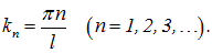
This is possible only for certain values of the wave vector:
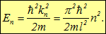
Since the energy of the particle is related to the wave vector, then
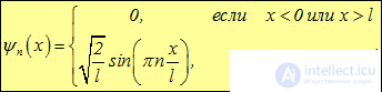
We have obtained the quantization of energy, that is, our "string," fixed at both ends, has started to sound, since distinct frequencies have appeared. Substituting the found allowed values of the wave vector into the expression for the wave function, we obtain it in the form
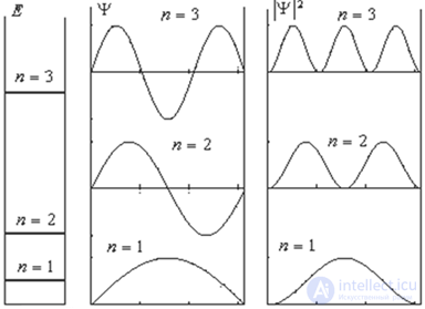
The meaning of the quantum number: it is one greater than the number of zeros of the wave function. The value of the constant
is determined from the normalization condition.
Fig. 4.8. Energy levels, wave functions, and the distribution of probability density along the coordinate x Note that the values Where, then, does the discreteness of energy levels, characteristic also of the atom, come from? Let us compare with a free particle: the equations are the same, but with different boundary conditions! Two formulations of the problem are possible here. In the first case, we investigate a state to which, in classical mechanics, an infinite motion would correspond (a scattering problem). Usually in such cases solutions are possible for any values of the energy (as one says, the spectrum is continuous). In the second case, we investigate a state to which, classically, a finite motion in a bounded region of space corresponds (a bound-state problem). The requirement that the wave function be finite throughout all of space leads to quantization of the energy. Let us stress: in this case the stationary equation has physically acceptable solutions not always, but only for certain values of the energy Example. Let us determine the spacing between neighboring energy levels Using expression (4.24) for the energy levels of a particle in a potential well, we find the energy spacing between neighboring levels
for large values of
Setting
This number by itself already tells us that classical formulas apply in the region of extremely high excitations. The spacing between the energies of neighboring levels is obtained by substituting into the formula for
In electron-volts these same characteristics have the values
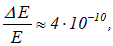
The relative spacing between the energies of neighboring levels is negligibly small:
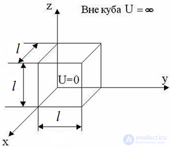
and hence in the classical limit the quantum discreteness is neglected. A particle in a three-dimensional potential well This is a generalization of the previous problem. The particle can move within a cubic volume with edge length
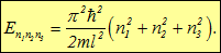
Such a wave function corresponds to the obvious fact that motions along the three axes are independent of one another, and each is described by the same one-dimensional wave functions as before. The energy, as is easy to guess, will equal the sum of the energies of motion along the axes x, y, z:
Fig. 4.9. Three-dimensional potential well The state of the system is now determined by three |
продолжение следует...
Часть 1 4. The Schrodinger equation
Часть 2 4.6. Bohr's correspondence principle - 4. The Schrodinger equation
Часть 3 - 4. The Schrodinger equation




 is a solution of equation (4.12), then
  is also its solution for any constant CA. Consequently, by choosing the constant A one can achieve satisfaction of the normalization condition (4.3).
 and
and  — are solutions of the Schrödinger equation, then the linear combination
  is also its solution (the superposition principle, that is, the basis of the phenomenon of interference).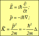
 there correspond in quantum mechanics the operators
  — multiplication by the vector
  , and
, and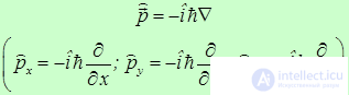
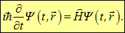


 , that is, the set of eigenvalues of the operator, determines its properties.
 . Here the role of states is played by ordinary radius vectors. Obviously, under rotation all vectors change except those parallel to the axis. These are precisely the eigenvectors of the rotation operator about the axis
  and
and  . An arbitrary rotation can be obtained by a combination of these three rotations. Accordingly, any radius vector can be represented as a linear combination of the three eigenvectors
  . The situation with other operators is essentially no different from the one described: knowing the set of eigenstates
  , any other state
  can be obtained with the help of a linear combination, that is, with the help of the superposition principle: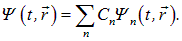
 of the corresponding operator
 of the corresponding coefficient in the expansion (4.17)).
 a measurement of
  will, with probability 100%, give the value
  (since in the expansion (4.17) only the coefficient with index
  is nonzero).
 of the total energy operator. According to what has been said, the equation has the form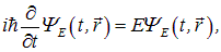
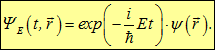
 , no longer dependent on time. It is called the wave function of the stationary state. The time dependence of stationary states is particularly simple — the same as for a free particle. It follows that in a stationary state the probability density does not depend on time. It is in this sense that the name "stationary" should be understood. Substituting solution (4.18) into the general Schrödinger equation (4.12), we obtain the stationary Schrödinger equation, that is, an equation for
  :
:
 . In operator notation it has the form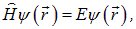






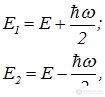
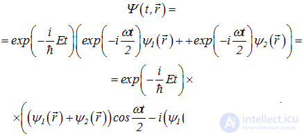
 it will pass into the antisymmetric state, and at the moment
  — it will return once again to the symmetric state. Consequently, the system oscillates between the symmetric and antisymmetric states with angular frequency
  . Here an analogy with classical physics can be seen: in the previously considered system of coupled oscillators similar eigenoscillations (normal modes) and beats arise.
 , and the derivatives with respect to y and z in the Laplace operator vanish. Equation (4.19) takes the form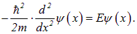
 , denoting
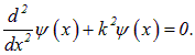


 and
and  are arbitrary). Analogy: the same kind of solutions describe the oscillations of a free string. Since waves with an arbitrary value of the wave number
  are possible, the energy of the particle (
 ) can also take any values, that is, in this case of free infinite motion — it is not quantized. For a particle moving in an arbitrary direction along an arbitrarily oriented wave vector
  , the same solutions hold, with the replacement
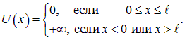
 and
and  . The particle cannot penetrate the region of infinite potential, and consequently
  outside the segment
  . Inside the well
  , and the stationary Schrödinger equation has the same form as for a free particle. The same solutions are obtained in the form of a superposition of standing (or traveling) waves, but unlike the previous case, boundary conditions are added. Namely, at the points
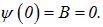
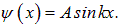




 , for which the boundary condition at the point
  is also satisfied, do not give new states. This is also evident from the expression for the energy (4.24), in which n enters squared, and from the expression for the wave function (4.25): a change in the sign of n will only change the sign of the wave function
  , which leaves the probability distribution
  unchanged.
 . As a consequence, a discrete energy spectrum of the system arises.
 for a particle in an infinitely deep potential well at large values of n. We shall use the result obtained to estimate the spacing between the energies of neighboring levels of the translational motion of nitrogen molecules at room temperature
  in a vessel. Let us take the mass of the molecule to be
  , and the linear size of the vessel
  . Let us compare the result obtained with the kinetic energy of the translational motion of the nitrogen molecules.
 . The average kinetic energy of the translational motion of nitrogen molecules equals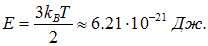
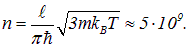
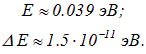
 the found expression for the quantum number: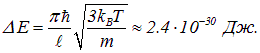
 . It is easy to verify that the general solution for the wave function can be represented as a product of one-dimensional wave functions obtained in the previous problem:

Comments