
Lecture
Это окончание невероятной информации про электрическое поле в вакууме.
...
data-auto-open loading="lazy" alt="1. The electric field in vacuum" >
(1.69)
symmetry. Functions of this kind appear whenever we deal with fields of spherical or axial symmetry, with the difference that in the first case  is the distance to the center of symmetry of the field, with which the origin of coordinates is made to coincide, while in the second
 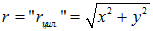 is the distance to the axis of symmetry of the field, along which the axis
  of the coordinate system is directed. Both of these cases can be treated in a uniform way.
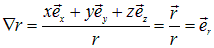
To begin with, let us calculate  .
.
Performing the differentiation, we obtain
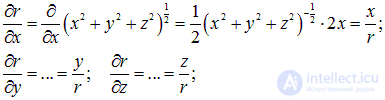
Now let us multiply each partial derivative by the unit vector of the corresponding axis and add the results
|
|
(1.70) |
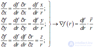
Let us now calculate the gradient of an arbitrary scalar function depending only on the magnitude of the position vector 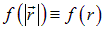 . In both cases
  is a composite function of the coordinates
  of the point: the function
  does not depend on them directly and independently, but through the mediation of the inner function
 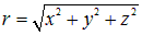 . According to the rule for differentiating composite functions
|
|
(1.71) |
Comparison shows that this is simply a particular case for  , when
  .
.
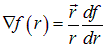
Thus, the general formula for the gradient of a scalar function depending only on the magnitude of the position vector has the form:
|
|
(1.72) |
In the particular case of the potential of the field  of a point charge located at the origin of coordinates, as it should be, we obtain
|
|
(1.73) |
We suggest deriving on your own the following useful relations:
|
|
(1.74) |
In the operator  in the first relation, the differentiation is carried out with respect to the coordinates
  of the point with position vector
  , while in the operator
  in the second relation — with respect to the coordinates of the point
  with position vector
  . To simplify the derivation, it is recommended to make the substitution
 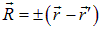 .
.
Часть 1 1. The electric field in vacuum
Часть 2 1.4. Flux of a vector. The Ostrogradsky–Gauss theorem for a
Часть 3 1.5. Application of Gauss's theorem for calculating the electric field
Часть 4 Appendices - 1. The electric field in vacuum
Часть 5 - 1. The electric field in vacuum



Comments