
Lecture
In previous chapters we studied oscillations in systems with one, or at most two, degrees of freedom. Now we turn to systems with an infinite number of degrees of freedom. Examples include oscillations in a gaseous medium, oscillations of solid bodies, of a stretched string, and so on. In all these examples, oscillations are possible at every point of the medium or body, which can be regarded as an oscillator. Neighboring oscillators are coupled to one another, so that processes of energy transfer between them are possible. In such cases one speaks of a propagating wave.
Oscillations of a string
Let us consider small oscillations of a string stretched with a force T along the x axis. Let the displacement of an arbitrary point of the string with coordinate x at time t be the vector  . We restrict ourselves to the simplest oscillatory process, in which all the displacement vectors
  at any moment of time are perpendicular to the x axis and lie in a fixed plane. Then the displacements of points of the string can be described by a single scalar function
  , as shown in Fig. 2.1.
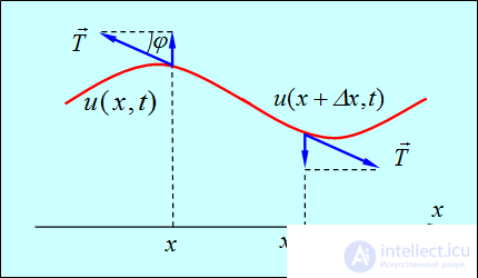
Fig. 2.1. Oscillations of a string
The tensions arising in the string are directed along the tangents to its instantaneous profile. We will consider small oscillations, in which the elongation of the string and the additional elastic forces arising from it can be neglected. Then the tension of the string can be considered constant for all moments of time t and points x. Let us isolate an element of the string lying between the coordinates x and  . Consider the point with coordinate x. The tangent of the angle of inclination of the force T acting on this edge of the element equals
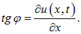
The vertical component of the force equals

Since the angle  is small,
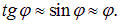
Then
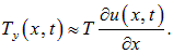
Similarly, the vertical component of the tension force of the string acting at the other end of the isolated element equals
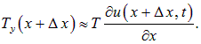
The resultant of these forces equals
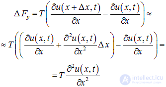
Note that the horizontal components of the tension force
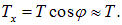
do not depend on the position of the point, and therefore their resultant equals zero. This means that, in the approximation under consideration, elements of the string move only in the vertical direction.
If the linear density (mass per unit length) of the string equals  , then the mass of the element equals

We write the equation of Newton's second law for the vertical displacement of the string element:
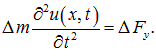
Substituting here the expression for  , we obtain the equation of motion of the string:
|
|
|
(2.1) |
This equation can be rewritten in the form:
|
|
|
(2.2) |
where
|
|
|
(2.3) |
Let us determine the dimension of the quantity  . The dimension of the force
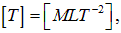
the dimension of the linear density of the string material
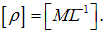
Hence the dimension of the quantity will be
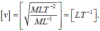
that is, the quantity has the dimension of velocity.
Oscillations in an ideal gas
Let us consider oscillations in a gas occurring along a single axis x. Unlike in the string, the gas particles are displaced here in the longitudinal direction, but we will denote the displacement by the same symbol u(x,t).
Let us consider an elementary volume of gas V0, bounded by cross-sections 1 and 2, located at the point with coordinates x and  (Fig. 2.2). The mass of gas in the volume equals
  , where
  — is the density of the gas, and S — is the cross-sectional area. In the equilibrium steady state the gas pressure equals
  .
.
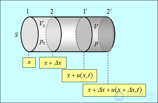
Fig. 2.2. Oscillations in a gas
During oscillations the isolated volume shifts to a new position between cross-sections 1' and 2' with coordinates

and

The volume of gas in the new position becomes equal to
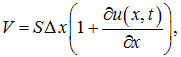
and the pressure in it — p. Let us find this pressure.
Oscillatory processes in gases occur quickly enough that the elementary volume can be considered not to have time to exchange heat with neighboring volumes. This means the process can be considered adiabatic. We write the equation of this process:

or
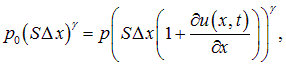
whence
|
|
|
(2.4) |
Here  — is the adiabatic index, depending on the type of gas. We also used the smallness of the derivative

for expansion into a series:
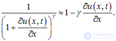
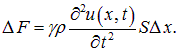
Let us now compose the equation of motion of the elementary volume. Its acceleration equals

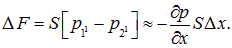
The force acting on the volume is determined by the difference of pressures in cross-sections 1' and 2':
|
|
|
(2.5) |
Substituting here the expression for the pressure p we find:
|
|
|
(2.6) |
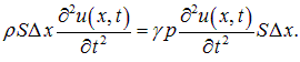
We now write Newton's second law
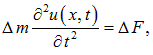
or
|
|
|
(2.7) |
After obvious cancellations this equation can be presented in the form:
|
|
|
(2.8) |
where
|
|
|
(2.9) |
The quantity has the dimension of velocity. The equation of oscillations of the gas coincided with the equation of oscillations of the string (2.2), although they describe processes in completely different physical systems.
Oscillations in solid bodies
Oscillatory processes in solid bodies are similar to oscillations in gases. Fig. 2.3 shows the longitudinal deformation of a solid body in the direction of the x axis.
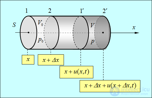
Fig. 2.3. Longitudinal oscillations in a solid body
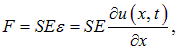
The relative deformation of the elementary volume under displacement u equals
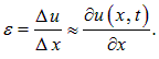
According to Hooke's law, this leads to the appearance of an elastic force
|
|
|
(2.10) |
where E — is the coefficient (Young's modulus) characterizing the stiffness of the medium. The resultant of the elastic forces acting at cross-sections 1' and 2' equals:
|
|
|
(2.11) |
Writing Newton's second law in the form:
|
|
|
(2.12) |
we find the equation of oscillations in a solid body:
|
|
|
(2.13) |
where
|
|
|
(2.14) |
The dimension of Young's modulus coincides with the dimension of pressure, so here too has the dimension of velocity.
Above we considered longitudinal displacements in a solid body. Unlike gases, elastic forces also arise in solids under shear deformation. The equation for such transverse oscillations has the same form (2.13), but instead of Young's modulus the expression for v contains the so-called shear modulus G:
|
|
|
(2.15) |
The mechanism of propagation of longitudinal and transverse oscillations is shown in Fig. 2.4 and 2.5.
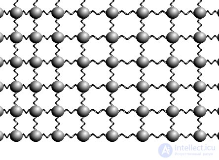
Fig. 2.4. Longitudinal waves in a solid body
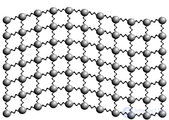
Fig. 2.5. Transverse waves in a solid body
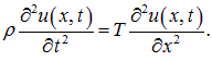
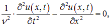
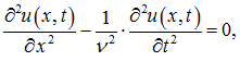
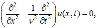
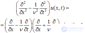
An equation of the type (2.2), describing the oscillations of various elastic media, is called the wave equation. Let us write it formally as:
|
|
|
(2.16) |
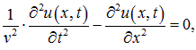
or
|
|
|
(2.16') |
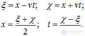
Let us now introduce, instead of (x, t), new variables:
|
|
|
(2.17) |
The derivatives with respect to the new variables are expressed by the standard rules for differentiating a composite function:
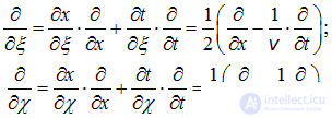
It follows from this that equation (2.16) in the new variables is written as:
|
|
|
(2.18) |
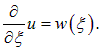
Since the derivative with respect to  is equal to zero,

does not depend on this variable and is therefore some function w of the variable  only:
only:
|
|
|
(2.19) |
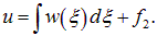
Let us now integrate this equation:
|
|
|
(2.20) |
The first term on the right-hand side is a function only of the variable  , which we denote as
  . The second term is a constant of integration. It does not depend on
  , being, therefore, a function only of the variable
  :
:

We have thus obtained that the solution of the wave equation has the form:

Substituting here the expressions (2.17), we return to the original variables (x, t):
|
|
|
(2.21) |
The functions f1 and f2 are completely arbitrary and must be determined from the initial and boundary conditions.
Let us discuss the physical meaning of the solutions obtained. We first restrict ourselves to the first term. Let

At the instant t = 0 the function f1(x) specifies the distribution of displacements (the profile of a string, the deformation of a solid body, the distribution of pressure or particles in a gas, etc.):
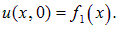
Suppose, for example, that this distribution has a maximum at the point  (Fig. 2.6).
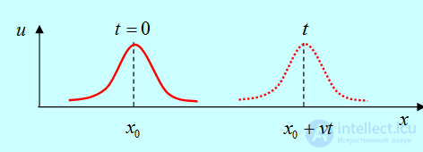
Fig. 2.6. Motion of the wave packet f1(x – vt)
Such a distribution is usually called a wave packet. At the instant t the maximum of the function  will still be at the point at which the argument
  equals
  , but now (at the instant
  ) the argument equals
  , thus:
  or
or  . In other words, in the time from 0 to
  the wave packet has shifted to the right by a distance vt, so that the maximum now falls at the point

It is easy to see that the wave packet does not change its shape during this displacement.
We see that the initial distribution moves to the right with velocity  . Similarly, the second term,
  , describes the motion of a wave packet to the left with the same velocity . The general solution (2.21) is a superposition of these two solutions.
In turn, any wave packet can be represented as a superposition of harmonic functions. Hence the special role of solutions of the wave equation of the form:
|
|
|
(2.22) |
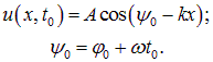
This solution describes a monochromatic wave, propagating to the right with velocity
|
|
|
(2.23) |
Indeed, expression (2.22) can be represented as
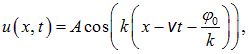
which is one of the countless possible specific realizations of the function f(x–vt) in (2.21). The quantity  is the angular frequency of the oscillations, and k is called the wave number.
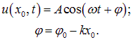
Suppose an observer is located at the point  and watches the oscillations of the medium at this point. He will find that the oscillatory motion occurs according to the law
|
|
|
(2.24) |
An observer at another point will also find harmonic oscillations of the same frequency, but with a different initial phase  . The further to the right the observation point, the greater the phase lag of the oscillations there. Correspondingly, the expression

describes a monochromatic wave propagating to the left.
Let us now carry out another thought experiment: let us "photograph" our wave at some given instant of time  (in the case of a vibrating string, no sophisticated instruments are even needed for this). In the snapshot we will see a periodic spatial structure:
|
|
|
(2.25) |
This structure has displacement maxima (Fig. 2.7) at points with coordinates xn, determined from the condition
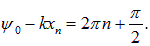
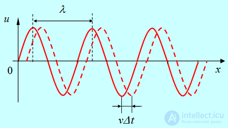
Fig. 2.7. Displacement of the points of the medium at the instant t (solid curve) and  (dashed curve).
The repetition period  of the same displacements in space is the distance between the nearest maxima:

We finally obtain:
|
|
|
(2.26) |
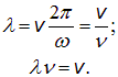
The quantity  is called the wavelength.
|
Wavelength is the minimum distance between two points of a wave at which the oscillations occur in the same phase. |
More precisely, the phases of the oscillations at two points separated from each other by  differ by
  , which, taking into account the periodicity of the sine and cosine, is the same thing as equality of the phases. Recall that such oscillations are most often simply called: in-phase oscillations.
If we "photograph" the wave at a nearby instant of time  , then in the snapshot the entire spatial structure will have shifted as a whole by a distance
  . The velocity v is called the phase velocity of the wave, since it is with this velocity that the maxima, minima, and in general all points with a given value of the phase move.
|
Phase velocity of a wave — this is the velocity with which the points of a wave that are oscillating in the same phase move. |
If, in the general case, we denote the phase of the wave at a point with radius vector  at the instant of time
  as
as  and introduce a surface of constant phase, at all points of which the phase has one and the same constant value
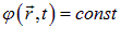 ,
,
then the phase velocity of the wave can be defined as follows: the phase velocity of a wave is the velocity of a point of the surface of constant phase. This is the velocity of a point belonging to the surface of constant phase; the surface itself is not stationary — its points move. In the simplest case of a plane wave of the form  the surface of constant phase is a plane perpendicular to the OX axis and moving along this axis with the phase velocity
  . Indeed:

Using (2.26) and (2.23), we find the relation between the characteristics of the wave:
|
|
|
(2.27) |
Here  — the frequency (in hertz) of the oscillations in the wave.
Fig. 2.8.
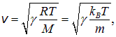
Let us give some numerical examples. A wave of compressions and rarefactions in a gas is a longitudinal elastic wave. Using the Mendeleev-Clapeyron equation for the state of a gas, we can write the speed of a sound wave in a gas (2.8) as:
|
|
|
(2.28) |
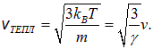
where M — molar mass, m — mass of a molecule, and T — absolute temperature of the gas. On the other hand, the root-mean-square velocity of gas molecules is also determined by its absolute temperature
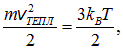
from which
|
|
|
(2.29) |
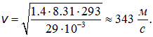
In other words, the speed of sound in a gas is, in order of magnitude, the same as the speed of thermal motion of the molecules. The molar mass of air is M=29·10-3 kg/mol, the adiabatic index is  . Substituting these values into (2.28), we find the speed of sound in air at room temperature (T = 20 °C = 293 K):
|
|
|
(2.30) |
The human ear perceives frequencies in the range from 20 Hz to 20 kHz. The corresponding wavelengths are:
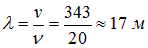
for the low frequencies and
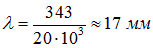
— for the high ones.
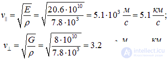
For steel, Young's modulus is E = 20.6·1010 N/m2, the shear modulus is G = 8·1010 N/m2, and the density is  . Accordingly, from (2.14), (2.15) we obtain the propagation velocities of longitudinal and transverse oscillations in steel
  :
:
|
|
|
(2.31) |
Finally, for water the role of Young's modulus is played by the quantity that is the inverse of the compressibility k=0.47·10-9 Pa-1. The density of water is  kg/m3. For the speed of sound in water we then obtain:
|
|
|
(2.32) |
Sound of the same frequency will have different wavelengths in water and in air. Thus, for  kHz we obtain the wavelength in water:
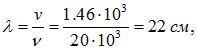
which should be compared with  mm in air.
Let us consider several examples for estimating the wavelength of a sound wave in various media.
Example 1. Ultrasound with a frequency of  MHz is used for diagnosing tumors in soft tissue. Let us find the wavelength of the ultrasonic wave in air and in soft tissue, where the speed of sound propagation is MHz = 1.5 km/s.
The wavelength of the ultrasonic wave in air
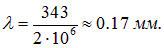
In soft tissue the wavelength of the ultrasonic wave is
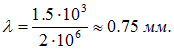
As we shall see later, the wavelength of any radiation imposes a natural limit on the size of objects that can be resolved with its help. This example shows that diagnosing tumors smaller than a millimeter using ultrasound is difficult.
Example 2. A bat uses ultrasound with a frequency of  kHz for orientation. Let us determine the size of obstacles that will certainly not be noticed by the bat, and answer the same question for dolphins, which also use these frequencies.
The wavelength emitted by the bat is
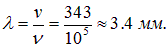
Obstacles smaller than this certainly cannot be noticed by the bat with the help of the emitted ultrasonic wave.
For dolphins the answer is different because of the different speed of sound propagation in water. The speed of sound in water is 1.46 km/s. Then
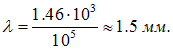
Thus, a bat can detect insects, while a dolphin can detect small fish.
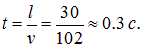
Example 3. A climber descending a sheer cliff is hanging on a rope 30 m long. His belaying partner sends him a signal by jerking the rope. Let us find how long it takes for the signal to reach the climber. The mass of the climber is 80 kg, the mass of one meter of the rope is 75 g.
Since we are given the linear density of the rope 7.5·10-2 kg/m and its tension force T = mg, then from formula (2.3) we find the propagation speed of the oscillations:
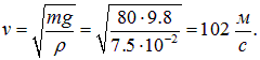
From this we determine the transit time of the signal:
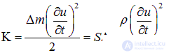
Let us consider a sound wave as an example. The volume element in Fig. 2.2 has kinetic energy:
|
|
|
(2.33) |
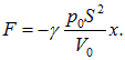
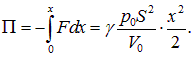
During its deformation, potential energy P is stored in this volume of gas. Considering the oscillations of the piston, we obtained expression (1.13) for the elastic force when the piston is displaced by a distance x:
|
|
|
(2.34) |
This law is analogous to Hooke's law for the elastic force during compression or extension of a spring. Consequently, the potential energy of the gas in this case is equal to
|
|
|
(2.35) |
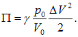
The product  is equal to the change in the volume of gas under the piston. Therefore (3.35) can be written as:
|
|
|
(2.36) |
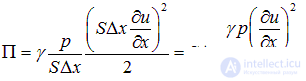
Let us apply this expression to the volume of gas in a sound wave. We denoted the pressure in the stationary state as  . The volume in the stationary state is equal to
  . The change in volume during the oscillations is equal to

We then obtain for the potential energy of this volume of gas:
|
|
|
(2.37) |
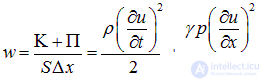
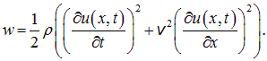
The sum of the kinetic and potential energy is equal to the total energy of this volume. We obtain the energy density w in the wave by dividing the total energy by the value of the volume:
|
|
|
(2.38) |
Taking into account that the phase velocity of the wave is equal to

we write (2.38) as:
|
|
|
(2.39) |
Exactly the same expression is obtained for a wave in a solid body (it does not matter whether it is longitudinal or transverse) and for a wave along a string.
Substituting here the solution (2.22)

for a monochromatic wave and taking into account the relation

we obtain identical expressions for the volume density of the kinetic and potential energies

so that their sum is
|
|
|
(2.40) |
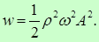
The energy density of the wave is different at different points in space and at different instants of time. Let us fix some point x and average the energy density at this point over time. The average value of the square of the sine is equal to 1/2. We then obtain that
|
the average value of the energy density is constant for all points of the medium and equal to
|
Thus, the medium possesses a total store of energy whose density is proportional to the density of the medium, the square of the angular frequency, and the square of the amplitude. Recall that for the oscillation of a system with one degree of freedom the energy of the oscillation was also proportional to the square of the frequency and the square of the amplitude of the oscillation, while in place of the density, — there stood the mass of the oscillating body.
If we return to expression (2.40) for the instantaneous value of the energy density, it is easy to see that any value of the energy density that we take, for example, its maximum

moves along the x axis with the phase velocity of the wave, velocity v. In other words, the wave carries energy. This energy is delivered, naturally, from the source of the oscillations. One can also introduce a vector of energy flux density

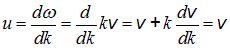
whose magnitude is numerically equal to the energy transferred per unit time through a unit area orthogonal to the direction of wave propagation. Note that the relations given above assume that the velocity  of energy transfer by the wave is equal to the phase velocity
  of the wave. This holds only in the case when there is no dispersion, that is, when the phase velocity of the wave does not depend on its wave number, namely, when
  .
.
Applications to a sound wave
The displacement of gas particles is described by the standard solution:

where the phase velocity is

Here p and  denote the pressure and density of the gas undisturbed by the wave.
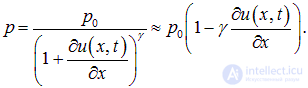
The displacement of the particles leads to the appearance of an excess pressure
|
|
|
(2.42) |
Here we used relation (2.4).
Taking into account that

formula (2.42) can be rewritten as:
|
|
|
(2.43) |
Note that the pressure oscillations are shifted by  relative to the displacement oscillations of the gas particles. At the maximum displacement
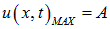
the pressure is equal to its stationary value, that is

Conversely, the pressure amplitude reaches its maximum at zero displacement of the gas particles.
|
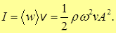
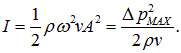
Intensity I of a wave — this is the average value of the energy flux density in it:
|
The intensity of the wave, just like the volume energy density, is proportional to the square of the amplitude.
Sound waves are customarily characterized by the loudness level L, measured in decibels (dB). The relation of the loudness level to the intensity of the sound wave is given by the formula:
|
|
|
(2.45) |
where
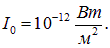
The choice of I0 is related to the threshold of hearing in the frequency range of 1,000 Hz – 4,000 Hz, to which the human ear is most sensitive. Thus, at I = I0 the loudness level is taken to be equal to zero. At wave intensities of order

the wave ceases to be perceived as sound, causing only a sensation of pain. This corresponds to a loudness level

Let us find the relation between the intensity of a sound wave, the excess pressure  , created by it, and the displacements of the gas particles. The amplitude of the pressure oscillations in the wave is equal to (see (2.43)):
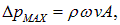
from which
|
|
|
(2.46) |
We also express the intensity of the wave in terms of the pressure amplitude:
|
|
|
(2.47) |
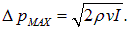
From this we find the excess pressure in the sound wave:
|
|
|
(2.48) |
Taking into account that the density of air under normal conditions is equal
продолжение следует...
Часть 1 2. Wave processes and elements of music theory
Часть 2 2.4. Standing waves - 2. Wave processes and elements of
Часть 3 2.5. Spherical waves - 2. Wave processes and elements of
Часть 4 - 2. Wave processes and elements of music theory













 (2.41)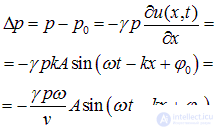

 (2.44)


Comments