5. Diffraction of light and waves

In a broader modern sense, diffraction is any deviation in the propagation of waves from the laws of geometrical optics (Physical Encyclopedic Dictionary, Moscow, Soviet Encyclopedia, 1983, p. 170).

Diffraction is observed for waves of any nature. Owing to diffraction, waves can penetrate into the region of geometrical shadow: sound can be heard around the corner of a house, radio waves can propagate far beyond the line of sight of a transmitting antenna, and a bright spot is observed at the center of the shadow cast by an illuminated disk.

In diffraction (as in interference), a redistribution of intensity occurs as a result of the superposition of waves. In essence, there is no fundamental difference between diffraction and interference: for historical reasons, the superposition of a finite number of waves is called interference, while the superposition of an infinite number of waves is called diffraction.

Owing to the vast range of technical applications, the diffraction of light is of particular importance. Observations of diffraction phenomena led wave optics to triumph over the corpuscular theory in the first half of the 19th century. In the limit of small wavelengths, the laws of wave optics reduce to the laws of geometrical optics. Consequently, deviations from the laws of geometrical optics are most pronounced when the dimensions of obstacles (various inhomogeneities) are comparable to the wavelength of light.

5.1. The Huygens—Fresnel Principle

The Huygens principle discussed earlier has the character of a geometrical rule. According to the Huygens principle, each point of a wave front can be regarded as an independent source of oscillations, and the result of the action of secondary waves can be found by constructing the surface enveloping these secondary waves. The French physicist A. Fresnel supplemented this principle, proposing to regard the wave disturbance at any point in space as the result of the interference of secondary waves from fictitious sources located on the wave front. These fictitious sources are coherent, and therefore can produce an interference pattern at any point in space, as a result of which the elementary waves can cancel or reinforce one another.

Fresnel's approach imparts a deeper physical content to the Huygens principle and also makes it possible to solve a number of problems that presented difficulties within the framework of the original Huygens principle.

Let us consider the surface of the wave front S (Fig. 5.1).

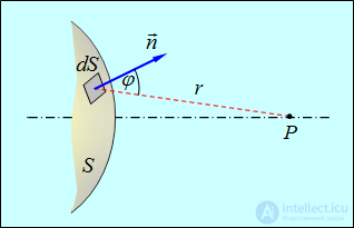
Fig. 5.1. Application of the Huygens—Fresnel principle to a spherical wave

In accordance with the Huygens—Fresnel principle

For a spherical wave, the amplitude decreases with distance r from the source as 1/r. Consequently, from each element dS of the wave surface an oscillation arrives at the observation point P

where — the amplitude of the light oscillation at the point of the wave surface where the element dS, is located, proportional to its area; — a coefficient that decreases as the angle between the normal n to the element dS and the direction from dS to the observation point P increases. The resultant oscillation at point P is the superposition of elementary oscillations dE, where the integral is taken over the entire wave surface S:

This relation represents the analytical expression of the Huygens—Fresnel principle.

In the general case, calculating the interference of secondary waves is quite complex and cumbersome, however for a number of problems, finding the amplitude of the resultant oscillation turns out to be possible using algebraic or geometric summation.

5.2. The Fresnel Zone Method

The Huygens—Fresnel principle, within the framework of wave theory, makes it possible to explain the rectilinear propagation of light. Let us determine the amplitude of the light wave at an arbitrary point P, using the Fresnel zone method. Let us first consider the case of an incident plane wave (Fig. 5.2).

Let the plane wave front F, propagating from a light source located at infinity, at a certain moment in time be at a distance OP – r₀ from the observation point P.

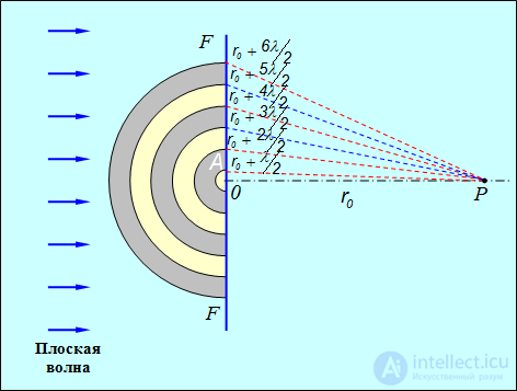
Fig. 5.2. Application of the Huygens—Fresnel principle to a plane wave: the Fresnel zones on the surface
of the plane wave front F are concentric rings
(for clarity, the image of the Fresnel zones is rotated 90°; this is how they appear from point P)

All points of the wave front, according to the Huygens—Fresnel principle, emit elementary spherical waves, which propagate in all directions and after some time reach the observation point P. The resultant amplitude of oscillations at this point is determined by the vector sum of the amplitudes of all secondary waves.

Oscillations at all points of the wave front F have the same direction and occur in the same phase. On the other hand, all points of the front F are located at different distances from the point P. To determine the resultant amplitude of all secondary waves at the observation point, Fresnel proposed a method of dividing the wave surface into ring-shaped zones, called Fresnel zones.

Taking the point P as the center, let us construct a series of concentric spheres whose radii start at and increase each time by half a wavelength . When intersected with the plane wave front F, these spheres yield concentric circles. Thus, ring-shaped zones (Fresnel zones) with radii etc. appear on the wave front.

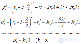
Let us determine the radii of the Fresnel zones, bearing in mind that , OA² = AP² – OP², that is

Similarly, we find

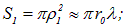
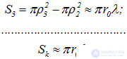
To estimate the amplitudes of oscillations, let us determine the areas of the Fresnel zones. The first zone (a circle):

the second zone (a ring):

the third and subsequent zones (rings):

Thus, the areas of the Fresnel zones are approximately equal, so, according to the Huygens—Fresnel principle, each Fresnel zone serves as a source of secondary spherical waves whose amplitudes are approximately equal. Moreover, the oscillations excited at point P by two neighboring zones are opposite in phase, since the path difference of the corresponding waves from these zones to the observation point P equals . Therefore, upon superposition these oscillations must mutually weaken one another, that is, the amplitude A of the resultant oscillation at point P can be represented as an alternating series

where A₁ — is the amplitude of oscillations at point P excited by the action of the central (first) Fresnel zone, A₂ — is the amplitude of oscillations excited by the second zone, and so on.

The distance from the m-th zone to the point P slowly increases with the zone number m. The angle between the normal to the elements of the zone and the direction to the point P also increases with m, consequently, the amplitude A_m of the oscillation excited by the m-th zone at point P, monotonically decreases as m increases. In other words, the amplitudes of oscillations excited at point P by the Fresnel zones form a monotonically decreasing sequence:

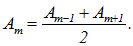
Owing to the monotonic and slow decrease of A_m we can approximately assume that the amplitude of oscillations from the zone with number m is equal to the arithmetic mean of the amplitudes of oscillations from the two neighboring Fresnel zones:

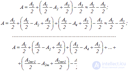
In the expression for the amplitude of the resultant oscillation, all the amplitudes from the even zones enter with one sign, and those from the odd zones with the other. Let us write this expression in the following form:

The expressions in brackets are equal to zero on the basis of (5.10), so that

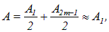
that is, the resultant amplitude created at the observation point P by the entire surface of the wave front is equal to half the amplitude created by the central (first) Fresnel zone alone. Thus, the oscillations excited at point P by the wave surface F, have the same amplitude as if only half of the first (central) zone were acting. Consequently, light propagates as if in a narrow channel, whose cross section is equal to half of the first (central) Fresnel zone — we have again arrived at the rectilinear propagation of a plane wave.

If, on the other hand, a diaphragm with an opening that leaves only the central (first) Fresnel zone open is placed in the path of the wave, the amplitude at point P will be equal to A₁, that is, twice the amplitude created by the entire wave front. Correspondingly, the intensity of light at point P will be four times greater than in the absence of an obstacle between the light source and point P. Surprising, isn't it? But there are no miracles in nature: at other points of the screen the light intensity will be weakened, and the average illumination of the entire screen when using the diaphragm will, as expected, decrease.

The validity of this approach, consisting in dividing the wave front into Fresnel zones, has been confirmed experimentally. Oscillations from the even and odd Fresnel zones are in antiphase and, consequently, mutually weaken one another. If a plate that blocks all the even or odd Fresnel zones is placed in the path of the light wave, it can be verified that the light intensity at point P sharply increases. Such a plate, called a zone plate, acts like a converging lens. Let us emphasize once again: Fresnel zones are mentally isolated regions of the surface of the wave front, whose position depends on the chosen observation point P. For a different observation point, the arrangement of the Fresnel zones will be different. The Fresnel zone method is a convenient way of solving problems concerning the diffraction of waves by various obstacles.

Two types of diffraction are distinguished. If the light source S and the observation point P are far from the obstacle, the rays incident on the obstacle and going to point P, form practically parallel beams. In this case, one speaks of diffraction in parallel rays, or Fraunhofer diffraction. If, on the other hand, the diffraction pattern is considered at a finite distance from the obstacle that caused the diffraction, one speaks of diffraction of spherical waves, or Fresnel diffraction.

5.3. Diffraction at a Circular Aperture and Disk

Similar diffraction phenomena can be observed when light passes through a small opening or, as is customarily said, from a complementary screen — a disk of the same size as the opening. Let a plane light wave be incident on a small circular opening of radius a (Fig. 5.3).

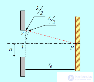
Fig. 5.3. Diffraction of light at a circular aperture

The plane front coinciding with the opening can be regarded as a set of fictitious sources emitting coherent waves, which will interfere at the observation point P. Let us divide the area of the opening into a number of ring-shaped Fresnel zones, for which we draw from point P a series of spheres with radii:

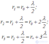
and so on.

If the number of zones fitting within the opening is even, then a dark spot will appear at point P. Indeed, the resultant amplitude of oscillations for 2, 4, ... 2m zones is respectively equal to

For small openings (small m) the amplitudes A₁ and A_m2+1 differ little from each other, so the resultant amplitude will be small, and a dark spot will appear at the observation point.

For an odd number of zones k = 2m-1 (m=1, 2, 3, ...) similar reasoning leads to the expression

that is, there will be a bright spot at the observation point.

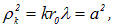
The number of Fresnel zones fitting within the opening depends on the distance and the wavelength :

from which the number of open zones is found to equal

Thus, for a given opening radius a and wavelength of the incident light the number of Fresnel zones k is a function of the distance between the opening and the observation point.

Calculating the amplitude of the resultant oscillations arriving at other points of the screen is more complex. From considerations of symmetry it follows that the interference pattern on the screen around the central bright (or dark) spot (depending on the parity of the number k) must have the form of alternating bright and dark rings centered at point P. The intensity of the maxima should decrease with distance from point P.

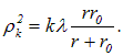
If the light source is located in front of the opening at a finite distance r from it, the calculation of the Fresnel zones becomes slightly more complicated: the zones are constructed not on a plane, but on a spherical front. We present, without derivation, the expression for the radii of the Fresnel zones in this case:

At

we arrive at formula (5.4) for a plane wave.

Let us now place between the incident plane wave and the observation point P an opaque disk of the same radius a — a complementary screen (Fig. 5.4).

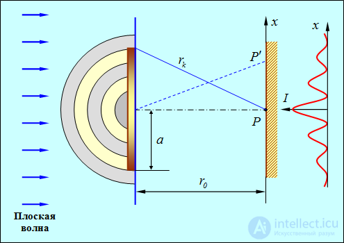
Fig. 5.4. Diffraction of light by an opaque disk: on the right is shown the distribution of screen illumination as a function of the distance x from the center of the screen.
The bright spot at the center (maximum value of the light intensity I) is followed by alternating minima and maxima, forming bright and dark rings

If the disk covers k of the first Fresnel zones, the amplitude at point P will be equal to

The expressions in brackets, as in formula (5.13), can be set equal to zero, that is

Thus, behind a small opaque disk

there will be a bright spot at the center of the screen. The larger the disk, the smaller, evidently, the amplitude A_k+1 and the weaker the illumination of the spot, that is, the less significant the diffraction. For a point P', displaced relative to point P in any radial direction, the disk will cover part of the (k + 1)-th Fresnel zone, while at the same time part of zone k will be uncovered. This will cause a decrease in intensity. At a certain position of point P' the intensity reaches a minimum. Consequently, in the case of an opaque circular disk, the diffraction pattern has the form of a bright central spot and alternating dark and bright concentric rings (see Fig. 5.4). The bright spot at the center of the geometrical shadow, predicted by S. Poisson in 1818, was put forward as a refutation of the wave theory of light. However, D. Arago proved experimentally that Poisson's conclusions correspond to reality and only confirm the wave theory and its predictions, which follow from the Fresnel zone method.

Example 1. On a diaphragm with a circular opening of diameter d = 4 mm, a plane light wave ( µm) is incident normally. The observation point is located at a distance b = 1 m on the axis of the opening. Let us determine how many Fresnel zones fit within the opening.

We use (5.16) with a = d/2 and r₀ = b:

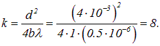
There will be a dark spot at the center of the pattern.

Example 2. A point light source ( µm) is located at a distance l = 1 m on the axis of a diaphragm with an opening of radius a = 1 mm. A screen is placed behind the opening. Let us find at what distance from the opening to the screen 3 Fresnel zones will be open for the center of the diffraction pattern.

We use formula (5.17):

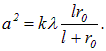
From this we find

At the center of the diffraction pattern, for k = 3, there will be a bright spot, and in accordance with formula (5.14) the amplitude of oscillations at this point will be equal to

If the diaphragm is removed, the amplitude will become equal to A₁/2, that is, the illumination (light intensity) will decrease by a factor of four.

5.4. Fraunhofer Diffraction from a Slit

Let a plane light wave be incident on an infinitely long slit. According to the Huygens—Fresnel principle, the illuminated slit can be regarded as a set of point coherent wave sources. Let us place a screen behind the slit, at a distance sufficiently large compared with the width of the slit. This condition means that onto a given point P of the screen falls a parallel beam of rays, deflected by an angle (Fig. 5.5).

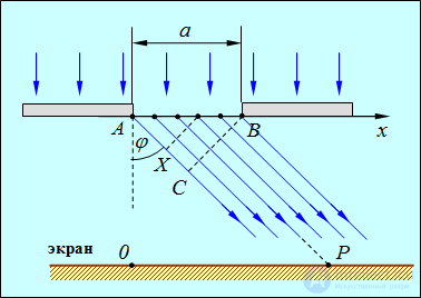
Fig. 5.5. Fraunhofer diffraction from a slit

The path difference of the extreme rays of this beam is determined from the triangle (angle ):

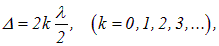
where a = AB — the width of the slit. If, when observed from point P, an even number of Fresnel zones fits within the slit (), then their contributions cancel one another, and a minimum of light intensity is observed at point P. Thus, the equation

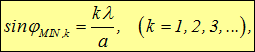
gives the condition for diffraction minima, where the angle — is the direction to the minimum with number k.

If the path difference of the extreme rays is equal to an odd number of half-waves

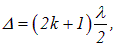
then, when observed from point P, an odd number of Fresnel zones fits within the slit. Each zone cancels its neighbor, and the one remaining zone sends light in the direction and forms a maximum. Therefore, the condition for maxima has the form

The considerations leading to expressions (5.21) and (5.22) are, generally speaking, approximate in nature, since we applied the Fresnel zone method for infinitely distant observation points, considering diffraction in parallel rays; however, as we shall soon verify, the condition for minima (5.21) turns out to be exact.

As for the central point 0 of the screen, located opposite the center of the slit, it receives a beam of undeflected rays orthogonal to the slit. All of them have the same phase, that is, they must reinforce one another. Therefore, in the condition for minima (5.21) the value k = 0, corresponding to point 0, is excluded.

The value k = 0 is also excluded from the condition for maxima (5.22), since it gives a value of the angle

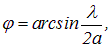
so that this maximum would have to be located between the central maximum and the first minimum

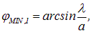
which is impossible.

After these qualitative considerations, let us study the diffraction pattern in more detail and obtain expressions that allow us to compare the light intensities at maxima of different orders. The resultant oscillation at some point P of the screen represents the superposition of oscillations propagating from the entire surface of the slit. In the case of Fraunhofer diffraction, the distance from the observation point to the slit can be considered approximately constant for small angles . The coefficient in formula (5.2) can also be considered constant if we limit ourselves to considering not too large diffraction angles . Let us denote by A₀ the total amplitude of oscillations excited by the slit at the central point 0 of the screen. Since the slit is infinitely long, let us divide it into strips of width dx so that, instead of integrating over the surface S (see formula (5.2)), we go over to integrating over the coordinate x along the width of the slit. Then the amplitude of oscillations excited by an element of the slit dx, will be equal to

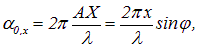
The amplitude of oscillations excited by this same element at any other point P will be the same. However, if this element is located at a point with coordinate x (we place the origin of coordinates at the extreme point A of the slit), then the secondary wave arriving from it at point P, will lead in phase the oscillation arriving at P from point A. The phase difference between the oscillations under consideration is formed along the path (see Fig. 3.5). If the initial phase of the oscillation excited at point P by the elementary area located at point A, is set equal to zero, then the initial phase of the oscillation excited by the area with coordinate x, will be equal to

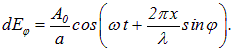
where — is the wave number of the light wave. Thus, taking (5.23) and (5.24) into account, we find the oscillation excited at point P by the element of the slit with coordinate x.

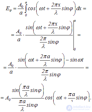
Let us integrate this relation over the entire width of the slit (0<x<a) and obtain the resultant oscillation excited at point P.

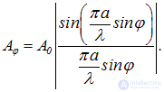
Thus, the amplitude of the resultant oscillation has the form

For point 0, lying opposite the center of the slit, the angle and A = A₀. This result follows, as we have seen, also from physical reasoning.

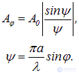
Let us find the position of the other maxima. To do this, let us represent the resultant amplitude in the form

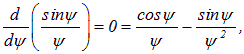
The amplitude has a maximum when the condition is satisfied:

or

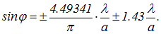
The obvious solution corresponds to the central maximum. The next root of equation (5.30), which can be solved only numerically, is equal to 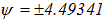. From this we find the condition for the first maximum:

From the approximate expression (5.22), for k = 1 we obtain a coefficient of 1.5 instead of the correct 1.43, which leads to an error of only 5 %. For the other maxima, agreement with the approximate formula becomes even better. The suspicious point

corresponding to the value k = 0 in condition (5.22), does not lead to an extremum of the amplitude (5.27), as should be expected.

At angles , satisfying the condition

the amplitude , as can be seen from (5.28), is equal to zero. This condition determines the position of the minima, as was obtained above in (5.21).

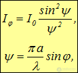
The light intensity is proportional to the square of the amplitude. Consequently, from formula (5.28) we obtain

where I₀ — is the intensity at the center of the diffraction pattern, I - is the intensity at point P, whose position is determined by the angle . Substituting here, we find the intensity I₁ at the first maximum:

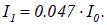
In other words, the intensity at the first maximum is almost 20 times smaller than at the central one. The intensity at the other maxima will be even smaller.

Thus, the central maximum gives the principal image of the slit. As a measure of its width, one can take the distance between the minima to the left and right of it. Using the condition for the first minima

and taking into account that for small angles

we obtain that the minima are seen at angles

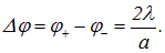
Therefore, the angular size of the central maximum is equal to

Similar formulas for openings of other shapes differ only by a numerical coefficient. From this a general conclusion follows for any optical instruments. If, using an optical instrument (a microscope, a spyglass, etc.), one attempts to distinguish two objects whose angular separation is equal to , this will be possible if

Here α is to be understood as the linear size of the opening of the instrument — its objective (if the objective has a diaphragm, then α — is the diameter of the diaphragm). Otherwise, the images of the objects (their central maxima) will fall practically at the same point, and the objects will be impossible to distinguish. To increase the resolving power of an instrument, one must either increase the diameter a of the objective, or use as short waves as possible. The latter is realized in electron microscopes.

5.5. The Diffraction Grating

Wide application in scientific experiments and technology has been found by diffraction gratings, which represent a set of parallel identical slits, spaced at equal distances, separated by opaque gaps of equal width. Diffraction gratings are manufactured using a ruling engine, which cuts lines (scratches) on glass or another transparent material. Where a scratch has been made, the material becomes opaque, while the gaps between them remain transparent and effectively act as slits.

Let us first consider the diffraction of light by a grating using the example of two slits. (As the number of slits increases, the diffraction maxima merely become narrower, brighter, and sharper.)

Let a — be the width of a slit, and b — the width of the opaque gap (Fig. 5.6).

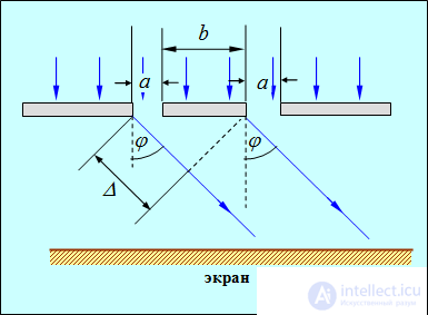
Fig. 5.6. Diffraction from two slits

The path difference of the two extreme rays is equal to

If the path difference is equal to an odd number of half-waves

then the light sent by the two slits, owing to interference of the waves, will mutually cancel. The condition for minima has the form

These minima are called secondary.

If the path difference is equal to an even number of half-waves

then the waves sent by each slit will mutually reinforce one another. The condition for interference maxima, taking (5.36) into account, has the form

This is the formula for the principal maxima of a diffraction grating.

Moreover, in those directions in which not a single slit sends out light, it will not be sent even with two slits, that is, the principal minima of the grating will be observed in directions determined by condition (5.21) for a single slit:

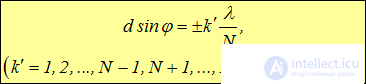
If a diffraction grating consists of N slits (modern gratings used in instruments for spectral analysis have up to 200,000 lines, with a period d = 0.8 µm, that is, of the order of 12,000 lines per cm), then the condition for the principal minima is, as in the case of two slits, relation (5.41), the condition for the principal maxima — relation (5.40), while the condition for the secondary minima has the form

Here k' can take on all integer values except 0, N, 2N, ... . Consequently, in the case of N slits, between two principal maxima there are (N–1) secondary minima, separated by secondary maxima that create a relatively weak background.

The position of the principal maxima depends on the wavelength l. Therefore, when white light is passed through the grating, all the maxima, except the central one, are decomposed into a spectrum, whose violet end is turned toward the center of the diffraction pattern, and the red end — outward. Thus, a diffraction grating represents a spectral instrument. Note that whereas a spectral prism deflects violet rays most strongly, a diffraction grating, on the contrary, deflects red rays more strongly.

An important characteristic of any spectral instrument is its resolving power.

where — is the minimum difference in the wavelengths of two spectral lines at which these lines are perceived separately.

Let us determine the resolving power of a diffraction grating. The position of the midpoint of the k-th maximum for wavelength

is determined by the condition

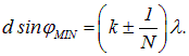
The edges of the k-th maximum (that is, the nearest secondary minima) for wavelength l are located at angles satisfying the relation:

Two close maxima are perceived separately if the midpoint of one maximum coincides with the edge of the other (Rayleigh criterion).

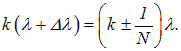
Thus, the midpoint of the maximum for wavelength

coincides with the edge of the maximum for wavelength l in the case where

From this we find

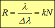
Consequently, the resolving power of a diffraction grating

is proportional to the order of the spectrum k and the number of slits N.